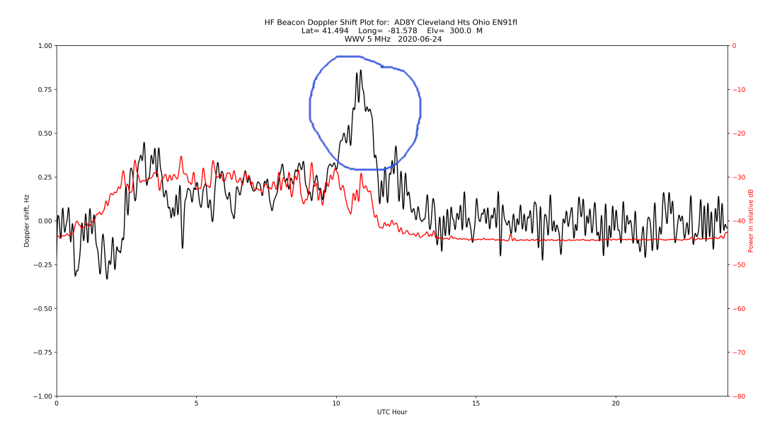
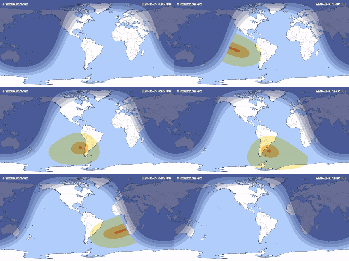
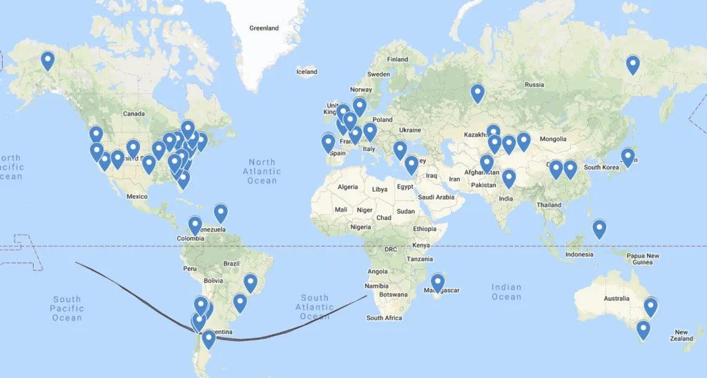
Changes in ionospheric electron density caused by space weather and diurnal solar changes are known to cause Doppler shifts on HF ray paths. For example, see Figure 7 in Boitman et al., 1999. As part of the WWV centennial, 50 stations collected Doppler shift data for the original Festival of Frequency Measurement, demonstrating the value of volunteer participation in collecting this data. This June, we request that all amateur radio stations, shortwave listeners, and others capable of making high-quality HF frequency measurements help us collect frequency data for the June 10 annular eclipse. Researchers will use the crowdsourced data to investigate the superimposed effects of auroral particle precipitation and the eclipse on Doppler shift.
All you need to collect data is an HF rig connected to a computer running open-source software. A precision frequency standard, such as a GPS-disciplined oscillator, is desired but not required to participate. All ham operators and shortwave listeners around the globe are invited to join in, even if your station is far from the path of totality. Last year's eclipse festivals included over 100 participants from 45 countries. The experiment will run from 7-12 June. All participants will receive QSL certificates and updates as the data is processed. This is a pilot experiment for HamSCI's Personal Space Weather Station project, which seeks to develop a global network monitoring the geospace environment.
This eclipse crosses the auroral oval. When observing Doppler shift, what combined effects do we observe from the aurora and eclipse?
What properties of the ionosphere are we able to measure by observing the variation in these HF propagation paths?
What effect will the annular eclipse have on these propagation paths?
How do various measurement techniques for understanding the path variation compare?
Is there volunteer interest in collecting data in the regions near totality for this eclipse?
Objectives
Promote international goodwill by working with citizen scientists around the globe
Measure Doppler shifts caused by space weather's effects on the ionosphere
Refine experimental procedures for future eclipse experiments
Develop digital signal processing for RWM
Times
Data recording starts: 07 June 2021, 0000 UTC
Data recording ends: 12 June 2021, 2359 UTC
Please begin measurements before the day's start time and end them after the finish time, if possible.
Beacons
The primary beacon for this experiment will be the Russian time standard station RWM on 9.996 MHz. If you are unable to receive it at your station, please try 10 MHz WWV or another station from this list. Experiment with your radio to see which stations are easiest for you to receive.
2) Collect data according to the instructions on this page: hamsci.org/doppler-instructions Use the instructions on collecting audio data in Audacity, not fldigi.
If you collected data for the December 2020 Eclipse Festival, the procedure is very similar, except that the local oscillator frequency must be included in the filename.
There will be an optional practice session on May 30th to select one or more beacon stations for the experiment. To participate, please listen for RWM (4.996 MHz, 9.996 MHz) and WWV (5 MHz, 10 MHz) on your radio and fill out the survey below. It's best to record around the same time of day as the eclipse (8 am UTC). If possible, please make a short recording with Audacity and upload it here.
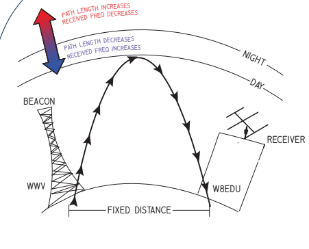
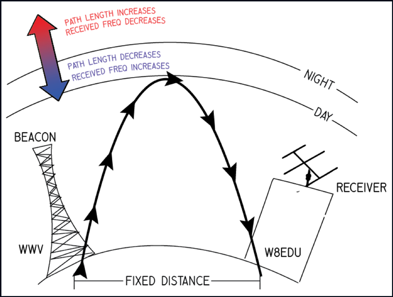
Radio signals provide a window into the changing ionosphere. The various signals from WWV, reflecting off the ionosphere, undergo changes in path length as the ionospheric electron density profile changes. This results in changes to the observed frequency of radio signals at receiving points, akin to the rise and fall in pitch of a passing train whistle.
Signals from radio station WWV reflect off the ionosphere in this illustration. Space weather affects how far a signal travels before it changes direction, and the receiving station detects this as a change in signal frequency.
Comparing the received radio signal with a precision local frequency standard, such as a GPS-disciplined oscillator, allows a user to measure these ionospherically induced frequency shifts. This measurement is prepared and recorded with open-source software. Numerous data sets recorded simultaneously from multiple locations offer information—when these data sets are examined both individually and collectively—about the ionosphere at the time the data are taken. This information includes the movements of traveling ionospheric disturbances and other important phenomena at various scales.
You can read more about how these measurements work here.
There are two ways to collect Doppler data from the audio output of your HF radio. One is to collect .CSV data using a frequency analysis program - this is best for long-term data collection. The other is to collect audio files, which is recommended only for short-term experiments such as eclipse festivals.
You will need:
An HF radio and antenna capable of receiving signals from time standard stations
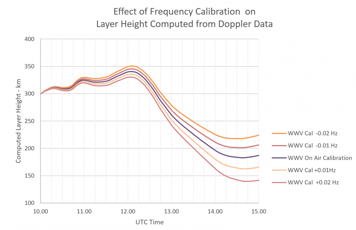
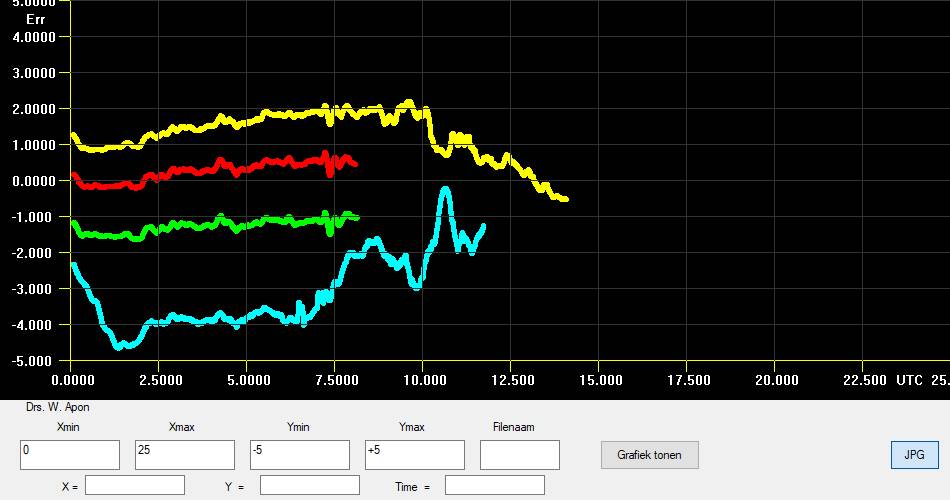
It is possible to collect data without a GPSDO, but your measurements will be much better with one. While you may be able to see trends in your data, you will not be able to make a quantitative estimation of layer height. As this chart by Steve Cerwin WA5FRF shows, a small error in your local oscillator frequency translates to a large error over time when estimating layer height:
Selecting a Beacon Frequency
You will want to record a beacon frequency that can be heard from your station. The examples on this page use 10 MHz. You can find a list of time standard stations here.
Radio time signal stations in the world with shortwave transmissions that you can use for Eclipse Festival of Frequency Measurement :
Africa :
None with shortwave transmissions.
African countries in the northern hemisphere : use RWM in Russia
African countries in the southern hemisphere : try to receive one of the time signal stations in South America,
else use RWM in Russia
Asia :
* BPM, China, Shaanxi, Pucheng (central China)
2.50 MHz, 5.0 MHz, 10 MHz, 15 MHz (Power in kW unknown for each frequency)
* HLA, South Korea, Daejeon
5.0 MHz (2 kW)
Europe :
* RWM, Russia, Moscow, Taldom (east of Europe)
4.996 MHz (10kW), 9.996 MHz (10kW), 14.996 MHz (10kW)
North-America :
* WWV, United States, Colorado, Near Fort Collins (central United States of America)
2.50 MHz (2.5 kW), 5.0 MHz (10 kW), 10.0 MHz (10 kW), 15.0 MHz (10 kW), 20 MHz (2,5kW), 25 MHz (2,5kW)
* CHU, Canada, Ontario, Ottawa (in the south east of Canada )
3.33 MHz (3 kW), 7.85 MHz (10 kW), 14.67 MHz (3kW)
Oceania :
None with shortwave transmissions.
Use WWVH in Hawaii or BPM in China
Pacific Ocean
* WWVH, United States, Hawaii, Kekaha (in the center of the north pacific ocean)
2.50 MHz (5 kW), 5.0 MHz (10 kW), 10.0 MHz (10 kW), 15.0 MHz (10 kW)
South America
* LOL, Argentina, Buenos Aires
10 MHz (2 kW)
* PPE, Brazil, Rio de Janeiro, Rio de Janeiro
10.0 MHz (1 kW)
* YVTO, Venezuela, Caracas
5.0 MHz (1 kW)
Recommendations for choosing the best radio station
1) use the nearest transmitter on your continent
2) use the frequency with the most power (in kW) if you can
3) for choosing the frequency to receive, try :
For continental and national radiocommunications we can summarize
- at night: bands from 3 MHz to 9 MHz,
- by day: bands from 5 MHz to 16 MHz.
For regional and departmental radiocommunications we can summarize
- at night: 0.3 MHz to 5 MHz band in Europe, 2 MHz to 6 MHz band in the tropics,
- by day: 0.3 MHz to 8 MHz band in Europe, 4 MHz to 12 MHz band in the tropics.
More detailed information by frequency band :
The propagation of electromagnetic waves depends of course on the medium but also on frequency. The ranges quoted below are given as an indication, the ionospheric propagation conditions being highly variable depending on the solar cycle, the time of year,the region of the world, the time of day, the circuits ... Below 4 MHz: Communications are generally only possible at great distance when it is dark between the place of transmission and reception, after the disappearance of layer D. The ground wave has a predominant function, especially in below 1 MHz. Excellent regional strip at the start and end of the day with a range of up to 600 km (up to 2,000 km depending on conditions). Local connections can take place within a radius of a few tens of kilometers. Communications possible without jump distance in NVIS radiation. 4 to 8 MHz: intercontinental communications are possible (over 4000 km) but reliable links can generally only take place between 200 and 3000 km. Local connections possible up to about thirty kilometers. Communications possible without a zone of silence in NVIS radiation (Sky Wave with Quasi Vertical Incidence) with a range of less than 400 km for the lowest frequencies of this portion of the spectrum. 8 to 12 MHz: Open 24 hours a day for continental communications. Jumping distance from 300 km during the day to 1,000 km at night. Intercontinental communication possible when it is dark between the place of emission and reception. 12 to 16 MHz: Band open during the day with a range of up to 2000 km at all times. Communications possible to the antipodes during favorable periods of the solar cycle. Jumping distance varying from 200 km during the day to 1,600 km at night.
Approach #1: Collecting .CSV Data With fldigi
We specifically request that you use the open-source software packagefldigi, version 4.1.13 or later. Its "frequency analysis" mode generates daily files of frequency deviations, automatically named "analysis_(date).csv." It will be in the directory /fldigi/temp/, or .fldigi/temp/, or some equivalent. You must use a recent version of fldigi, or your data will be overwritten.
Download fldigi, install it, verify that it's working correctly. Find the "frequency analysis" module in the "op mode" pulldown menu.
Tune your radio (in AM mode) to a time standard station on 10 MHz, and determine which you can easily measure.
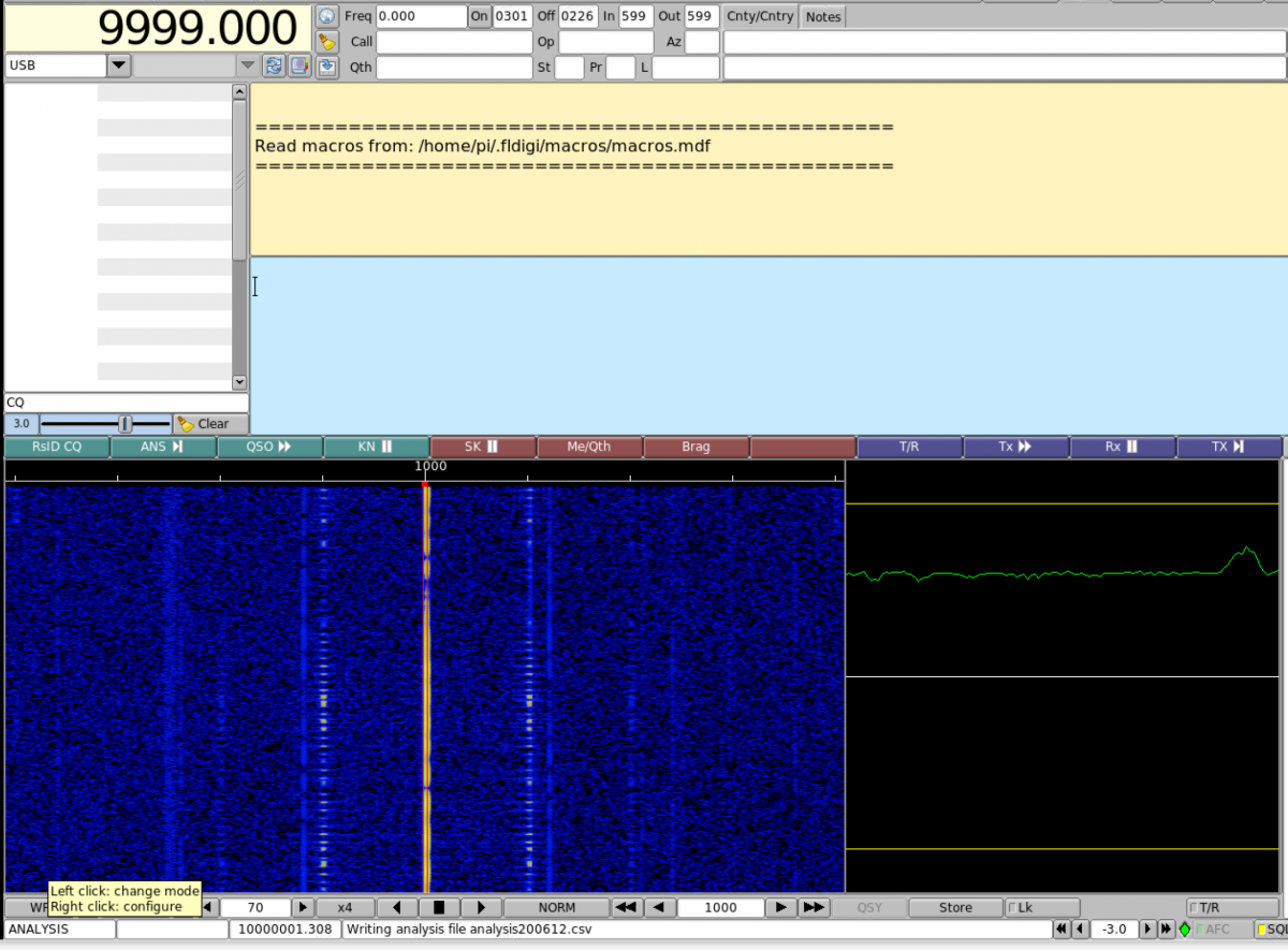
Set your receiver's mode to USB (upper sideband) and tune to a frequency 1kHz below the carrier. For 10 MHz, tune to 9.999 MHz (9999.000 kHz - see image) and listen for the 1000 Hz tone.
In fldigi, make sure that the tuned frequency in the upper left-hand corner is the same as your radio's frequency. To change it, click on the top half of a digit to increase it or the bottom half to decrease it.
Look for the 1000 Hz line on fldigi's waterfall. Click the cursor there or use the offset frequency box at the bottom of fldigi's screen. You must set the number in the box at the bottom of the screen to exactly 1000. (If fldigi doesn't take this input properly, try starting the recording and then setting to 1000.)
In fldigi, select the "Op Mode" menu and select "Freq Analysis" mode.
Look for "writing CSV file" on the lower line of fldigi, toward the left. If you have a clean signal and see only one carrier, you should see a nice plot at the end of the day. If you see multiple carriers, more detailed Doppler information may be needed.
Now, leave fldigi alone. While collecting data, leave your radio alone and make sure your computer is not shut down by an automatic update.
At the end of your recording period, close fldigi. The file "analysis.csv" should be in your /fldigi/temp/ directory. Alternatively, they may be under "/fldigi.files/analysis". In MacOS, they are in the hidden directory ~/.fldigi/analysis - to find them, you must unhide the files using CMD + SHIFT + . in Finder. At the end of the data collection period, you should have one analysis-*.csv files for each day of data recording. Please rename these files by adding your name or callsign: e.g., analysis_200620 - W8EDU.csv. Do not edit the content of the files.
Approach #2: Collecting Audio Data With Audacity
Note: This approach is for short-term data collection, such as during eclipse festivals. For long-term data collection, we recommend using fldigi as described above.
1) Connect your radio to your computer sound card.
If you're working in a language other than English, you can set it using Edit > Preferences > Interface Options.
3) Set up Audacity metadata.
Download this XML template and make a note of the directory it downloads to: EclipseTags.xml
Under Edit>Metadata, click "Load" and select the file, then edit it to fit your station.. (You can also add metadata manually using the list below.)
In Audacity, go to Edit > Metadata and fill in the following metadata fields:
Under Artist Name, put your callsign. (If you are a shortwave listener and not a ham, please use your name or SWL callsign.)
Under Album Title, put the name of the event - e.g., "December 2020 Eclipse."
Under Year, 2020.
Under Genre, put your radio model.
Add and fill in the following metadata fields.
Email Address
Rig
Antenna
Sound Card
Frequency
AGC (on or off)
Latitude (please use decimals, not minutes and seconds!)
Longitude
Elevation (m)
Time zone (Format example: UTC-05:00)
Grid Square
Country
IMPORTANT:If you have multiple radios collecting data simultaneously under a single callsign, add a hyphen and station number for each station wherever you would otherwise use the callsign. For example, if station W8EDU is running data collection simultaneously on a Flex radio and an Icom radio, they should label one as W8EDU-1 and the other as W8EDU-2, include a comment in the metadata for each station explaining that the operator ran multiple stations, and make sure that the metadata is correct and complete. This will make it much easier to sort through the data from the experiment during the analysis phase.
Hit "Save" and save the XML file, then hit "Set Default."
Check the box that says "Don't show this when exporting audio," then hit "OK."
4) Set recording preferences.
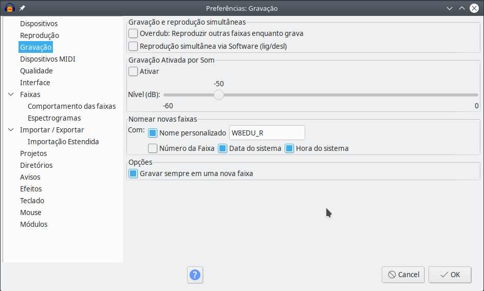
Open the Recording tab under the Preferences menu (Edit > Preferences > Recording). Uncheck "Play other tracks while recording" and check "Record on a new track" and "Detect dropouts."
For example, the station W8EDU is in Eastern Standard Time (UTC - 05:00), which corresponds to the letter R, so the correct custom track name will start with "W8EDU_R_". (If you're in a fractional timezone, use the letter J; this will flag your dataset for manual processing based on your location.)
Add your radio's local oscillator frequency. For example, if W8EDU is tuned to 9.999 MHz to listen for 10 MHz WWV, the Custom Track Name Field should read "W8EDU_R_9999kHz_". If W8EDU is tuned to 9.995 MHz to observe RWM at 9.996 MHz, the Custom Track Name Field should read "W8EDU_R_9995kHz_". This instruction has been added for the June 2021 Eclipse Festival, and is not currently shown in the screenshots below.
Make sure the boxes for "System Date" and "System Time" are also checked. When you're done, the window should look like this:
Under "Quality," set "Default Sample Format" to 16 bits. Set "Default Sample Rate" to 8000 Hz (unless your receiver requires a higher rate, as described in Step 2 above).
Go to "Devices" in the Preferences menu and make sure you are recording from your radio, as opposed to your computer's microphone or another source.
When done, click OK.
5) Set recording settings and make a test recording.
Set your recording to Mono (1 channel) on the pulldown menu in the middle of the top toolbar.
Make sure your project rate is set to 8000 Hz from the pulldown menu in the bottom left corner of the screen.
Set your audio input to the sound card connected to your radio. The device names will vary. You may have to experiment to make sure the source you're recording from is the correct one.
Hit the record ⬤ button; you should see the first track start recording, with the correct track name and timestamp. If the track name is not correct, try rebooting your computer and recording again.
Hit stop ⏹️, then record ⬤ again. This time, you should see a second track appear. The name on each track will correspond to its start time.
Note the "Disk space remaining for recording" at the bottom of your screen. One week of recording is 168 hours, so you may need to pause and restart data collection during the experiment. The estimate also may not be entirely accurate. Check Audacity's documentation on recording length here.
6) Save the project.
Make sure to stop ⏹️ the recording before you continue.
Save the project (File > Save). This will let the computer hang on to your settings. You may see a window asking if you want to save the project even though it has no tracks in it: click OK.
7) Check to make sure your WAV files save correctly.
Create a directory to save your files to according to the following convention: "<Callsign>_Eclipse_Dec2020". For example: W8EDU_Eclipse_Dec2020. (If you're running simultaneous data collection on multiple radios, use the hyphenated identifier described in Step 3.)
Go to File > Export > Export Multiple. Select the directory that you want to save your files to. Under "Name Files", make sure the option "Using Label/Track Name" is selected.
Click "Export." You should get a dialogue box confirming that each track has been saved to its own WAV file. (Note: If your files are too large to export, see the FAQ below.)
When these are done, you can delete your test tracks by clicking the X in the upper left hand corner of the track.
When you open the directory, you should see the artist and album metadata. Confirm that your filenames are in the correct format: "W8EDU_R_9.999MHz_2020-10-23_22-36-18.wav"., for example.
You should record your data on a drive that has at least 10 GB of free space. If you are running Windows, navigate to your data directory and activate compression: Properties -> General -> Advanced -> Compress contents to save disk space. (See screen shot below).
8) Optional: Calibrate Audio Output for the .WAV File Record
We're interested in collecting amplitude data where possible; you can read more about it here. If your radio has an automatic gain control (AGC) circuit that can be disabled, and a separate RF gain control, you can also collect amplitude data. It's not enough to just turn the AGC off, though; you have to set the RF gain to an appropriate level. Otherwise the audio level will be nearly a constant level regardless of the signal strength, and the data may be compromised. Once the AGC is turned OFF the receiver’s RF gain control must be set so that the audio level gives measurable amplitudes that never go full scale, clip, or limit. This will require preliminary testing to be sure the maximum signal strength does not overdrive the sound card input. If your radio does not fit these requirements, skip to Step 9 below.
Here is a method to set up the receiver:
With AGC enabled, set up the radio to produce the 1000 Hz tone in USB mode by tuning the radio 1 kHz below the carrier frequency (e.g., 9.999 MHz for a 10 MHz carrier).
Set the receiver volume control for a comfortable listening level using the radio’s normal speaker or headphones. It should be loud enough to be above the no-signal receiver noise but not so lout that it causes distortion.
Set the recording level in Audacity to get approximately 1/4-1/2 full scale recording level, or at the level that leaves about 6 dB to 10 dB of headroom below full scale.
Turn the receiver AGC OFF.
Use the RF gain control to set the audio output to the same level as with the AGC ON.
Make a day-long recording and examine the record. If the levels reached full scale at any time during the recording, reduce the RF gain control and try again. The idea is to have enough RF gain get measurable signal levels even during the weakest part of the day but not so much that the amplitude at the strongest part of the day hits or flattops at full scale.
Once the RF gain is set it must not be changed while recording eclipse data.
When submitting your data survey below, make sure to confirm that you performed this procedure.
9) All set!
Now you should be all set to collect data! If you need to restart data collection at any time, hit the stop recording button and repeat Step 7 above.
Once you're all set, your setup should look something like this:
Analyze Your Data
You can plot your data over time to see geophysical trends. If you are receiving a clear signal, the sunrise should show up clearly in your frequency data.
You will see variation day to day. If you plot data over a long period, you will see the morning peak shift with the changing length of day.
A good way to check the fidelity of your data: recruit friends nearby to take data on the same frequencies. This will help separate out local noise in your environment from signals that are geophysical in nature. In the plot below, all the stations are within 5km of one another, and the three stations on the top all have GPSDOs. (Image credit: Wim PA0SLT)
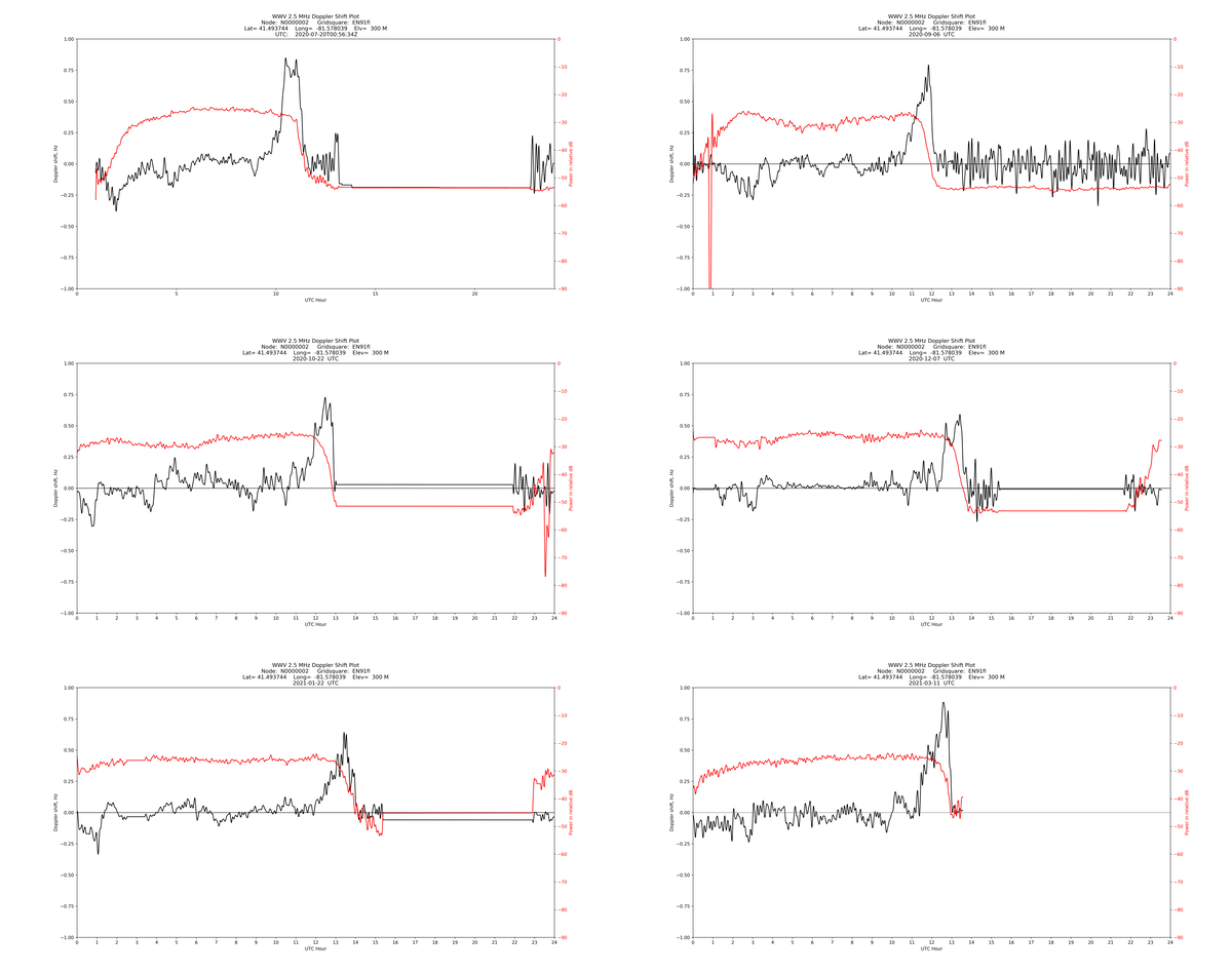
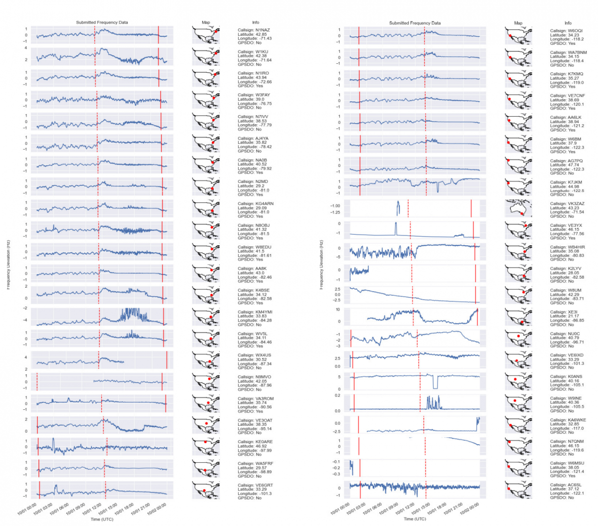
You'll see a lot of regional variation as well. Here's a plot of data taken during the original Festival of Frequency Measurement. You can read about the analysis of the data here.
Frequently Asked Questions
Q: What will this data be used for?
A: This data will be analyzed by members of the HamSCI organization. The data and results will be made public, as we did for the orignal Festival of Frequency Measurement.
Q: If I'm having trouble getting data collection to work, can you help me? A: Yes. Email [email protected] and we will help you get your radio set up.
Q: Can I use a program other than Audacity to make my measurements? A: Yes, but we cannot provide assistance for other programs. We also like Spectrum Lab, though.
Q: How can I check the metadata on my WAV files?
A:Most metadata tools won't show the nonstandard fields that we added, but you can use mediainfo if you want to see them. It has a nice command line interface, too.
Q: Can you still use my data if I can't record for the entire period? A: More data is always better, but if you need to take your radio back for part of the event (e.g., to run a traffic net) or experience a data interruption, then we're still interested in your data. Just be sure to stop recording before retuning your radio, tune back to 9.999 MHz before you start it up again when you're ready to resume collecting data, and leave us a note when you submit it.
Q: Will you accept other forms of data? A: Yes, although we can't guarantee we'll be able to use it.
Q: I can collect data for the experiment, but my Internet connection is so slow there's no way I'll be able to upload it to you. Can I submit it another way? A: Yes! Email me at [email protected] and I'll mail you a thumb drive.
Q: Audacity says my recording is too large to export as a WAV file. Why is this happening, and what can I do? A: WAV files are limited to 4 GB because the filesize is indicated in the header by a 32-bit unsigned int. Audacity will give you another chance to export. Select "Other uncompressed files," then under "Header," select "WAV(NIST/Sphere)." This will use a different header format, but your data should be the same, and can be uploaded as long as it is less than 32 GB.
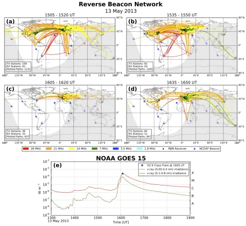
Solar flares and geomagnetic storms can significantly impact the ability to commicute on the medium and high frequency (300 kHz - 30 MHz bands). Solar flares cause radio blackouts due to collisional absorption from enhanced D-region ionization, especially on the lower frequencies. Geomagnetic storms can cause large-scale depletions of ionospheric densities that can reduce the maxium usable frequency (MUF) on a global scale. These impacts can be observed in large-scale amateur radio networks such as the Reverse Beacon Network, WSPRnet, and PSKReporter.
Publications
Frissell, N. A., Miller, E. S., Kaeppler, S. R., Ceglia, F., Pascoe, D., Sinanis, N., Smith, P., Williams, R., and Shovkoplyas, A. (2014), Ionospheric Sounding Using Real-Time Amateur Radio Reporting Networks, Space Weather, 12, 651– 656, https://doi.org/10.1002/2014SW001132.
Frissell, N. A., Vega, J. S., Markowitz, E., Gerrard, A. J., Engelke, W. D., Erickson, P. J., et al. (2019). High-frequency communications response to solar activity in September 2017 as observed by amateur radio networks. Space Weather, 17, 118– 132. https://doi.org/10.1029/2018SW002008.
Registration is now open for the 2021 HamSCI workshop. A full schedule of speakers and registration information can be found on the HamSCI Workshop 2021 website. The workshop will be held in a virtual format on Friday and Saturday, March 19-20. The University of Scranton will serve as host for the Zoom webinar, sponsored by the National Science Foundation (NSF), that will include addresses by guest speakers, poster presentations and demonstrations of relevant instrumentation and software. The theme of this year’s workshop is midlatitude ionospheric science.
The workshop will also serve as a team meeting for the HamSCI Personal Space Weather Station project, which is a NSF funded project awarded to University of Scranton physics and electrical engineering professor Nathaniel Frissell, Ph.D. The project seeks to harness the power of a network of licensed amateur radio operators to better understand and measure the effects of weather in the upper levels of Earth’s atmosphere.
The workshop’s keynote address on the “History of Radio” will be given by Elizabeth Bruton, Ph.D., curator of technology and engineering at the Science Museum of London. She will discuss the history, science, technology and licensing of radio amateur communities from the early 1900s through to the present day, exploring how individuals and communities contributed to “citizen science” long before the term entered popular usage in the 1990s. Dr. Bruton has been a non-licensed member of Oxford and District Amateur Radio Society since 2014 and their web manager since 2015.
J. Michael Ruohoniemi, Ph.D., professor of electrical and computer engineering at Virginia Tech and principal investigator of the Virginia Tech SuperDARN Initiative, will review the physics of the midlatitude ionosphere and discuss ways in which the amateur radio community can contribute to advancing scientific understanding and technical capabilities. Joe Dzekevich K1YOW, an amateur radio citizen scientist who recently published his work in CQ Magazine, will present “Amateur Radio Observations and The Science of Midlatitude Sporadic E.” The event will also include virtual oral presentations by researchers from NASA Goddard Space Flight Center, MIT Haystack Observatory, the University of Oslo, the University of Bath, Case Western Reserve University, Dartmouth College. the University of Alabama, Clemson University, the New Jersey Institute of Technology and The University of Scranton, among others.
University of Scranton students Veronica Romanek (KD2UHN), Hampton, New Jersey; Cuong Nguyen, Ashley; and M. Shaaf Sarwar (KC3PVF), Lahore, Punjab, are among the iPoster presenters. Participation is free thanks to support from the National Science Foundation and The University of Scranton.
Posters and presentations at the HamSCI workshop are made for community discussion and for exploration of new possibilities. Please note that these materials are not peer-reviewed.
The annual HamSCI Workshop will be held virtually this year March 19-20, 2021 using Zoom hosted by The University of Scranton and sponsored by the National Science Foundation. The primary objective of the HamSCI workshop is to bring together the amateur radio community and professional scientists. The theme of the 2021 HamSCI Workshop is midlatitude ionospheric science. We welcome submissions related to development of the Personal Space Weather Station, ionospheric science, atmospheric science, radio science, space weather, radio astronomy, and any science topic that can be appropriately related to the amateur radio hobby. We especially encourage subimissions related to this year's meeting theme of midlatitude ionospheric physics, but will also accept abstracts outside of this theme and otherwise appropriate. To submit an abstract, please fill out the on the HamSCI Workshop 2021 page at http://hamsci.org/hamsci2021.
Abstract: The midlatitude portion of the ionosphere is located roughly between 30° and 60° magnetic latitude, where the vast majority of radio amateurs operate. The midlatitude ionosphere has historically been considered less ‘active’ than the high-latitude auroral regions or the low-latitude equatorial zone and has received less scientific attention. However, the bulk of humanity lives at these latitudes and major vulnerabilities to space weather disturbance are found there. Some will be well-known to radio amateurs operating HF communications links. Increased interest in the midlatitude ionosphere has spurred the deployment of new observational facilities such as the midlatitude component of SuperDARN and the Personal Space Weather Station. In this tutorial, Dr. Ruohoniemi will present a review of the physics of the midlatitude ionosphere, discuss recent advancements and open questions at the frontiers of research, and consider means by which the amateur radio community can contribute to advancing scientific understanding and technical capabilities.
Bio: Dr. J. Michael Ruohoniemi is a professor of electrical engineering at Virginia Tech and Principal Investigator of the Virginia Tech Super Dual Auroral Radar Network (SuperDARN) Laboratory. Dr. Ruohoniemi earned his B.S. from the University of King's College and Dalhousie University, Nova Scotia in 1981 and his Ph.D. from the University of Western Ontario in 1986. After graduation he joined the team at the Johns Hopkins University Applied Physics Laboratory that developed HF radar into the SuperDARN concept to study the auroral (high-latitude) ionosphere. As a faculty member at Virginia Tech, he led a consortium of universities in building a chain of SuperDARN radars at midlatitudes across the U.S. His scientific publications now have over 9,700 citations. Today, 12 of the more than 30 radars in the SuperDARN network make continuous observations of the midlatitude ionosphere in both hemispheres, and these observations have been instrumental in advancing midlatitude ionospheric science in numerous studies.
Abstract: Amateurs may ask, “Why do we see Sporadic E like propagation in November and December, when many of the variables like UV radiation and solar exposure are at a minimum, unlike the very active sporadic-E summer months?” How are sporadic-E transatlantic VHF communications possible between North America and Europe? In his tutorial, Joe K1YOW will explain what Sporadic E is, how amateur operators use Sporadic E to enable long-distance VHF communications, current theories of Sporadic E formation, and how we might be able to better understand Es formation by examining amateur radio propagation logs. Joe’s studies of Sporadic E using amateur radio have been published both in QST (2017) and CQ Magazine (2020).
Bio: Joe Dzekevich, K1YOW, was first licensed in 1962 and currently holds an Amateur Extra Class license. He graduated from Northeastern University in 1977 with a B.S. in Industrial Technology and holds a M.B.A. from Clark University (1985). Joe is currently a retired Reliability Engineering Fellow who has worked for Bell Telephone Labs, Digital Equipment Corporation, Chipcom/3Com and Raytheon. Joe is also a senior member of the IEEE Reliability Society, where he held various offices in the local IEEE Boston Reliability Chapter and developed and taught many of the chapter’s courses. He is a member of NVARC (Nashoba Valley Amateur Radio Club), the ARRL, and HamSCI. He has always been interested in radio propagation, starting back in 1965 where he subscribed to the CRPL (Central Radio Prediction Lab) Ionospheric Predictions, where one used monthly CRPL prediction maps to chart predicted E-Layer and F-Layer radio paths.
Abstract: This talk will explore developments in the history, science, technology, and licensing of radio amateur communities from the early 1900s through to the present day, exploring how individuals and communities contributed to “citizen science” long before the term entered popular usage in the 1990s. I will also explore how these community-led developments can inspire the next generation’s interest in science, technology, engineering, and mathematics (STEM), citizen science, and amateur radio.
Bio: Dr Elizabeth Bruton is Curator of Technology and Engineering at the Science Museum, London, specializing in the history of communications. Prominent aspects of this role include curator of “Top Secret: From ciphers to cyber security” exhibition, which explored over a century’s worth of communications intelligence through hand-written documents, declassified files and previously unseen artefacts from the Science Museum Group's and GCHQ’s historic collections, and serving as co-Investigator on the “Electrifying Women: Understanding the Long History of Women in Engineering”, a nine-month Arts & Humanities Research Council (AHRC) project with Professor Graeme Gooday at the University of Leeds. Dr Bruton holds three degrees: a BAI in Computer Engineering from Trinity College, Dublin (2004); an MSc in history of science from the University of Oxford (2005) with a dissertation on “Marconi Wireless Telegraphy in the British Army during World War One”; and an AHRC-funded Collaborative Doctoral Award PhD with BT Archives and IET Archives at the University of Leeds on “Beyond Marconi: the roles of the Admiralty, the Post Office, and the Institution of Electrical Engineers in the invention and development of wireless communication up to 1908” (2013). Last and definitely not least, Dr Bruton has been non-licensed member of Oxford & District Amateur Radio Society since 2014 and their web manager since 2015.
Opening Remarks & Oral Session I
Personal Space Weather Station Engineering & Science Chair: Dr. Nathaniel Frissell W2NAF; Zoom Moderators: Bill Liles NQ6Z & Diego Sanchez KD2RLM
David M. Witten, III KD0EAG, Frances Bonte KE8HPA, & Hyomin Kim KD2MCR
TAPR; DeSales High School, Columbus, OH; New Jersey Institute of Technology
11:40 AM
1540z
Break
Oral Session II
Personal Space Weather Station Engineering & Science Chair: Dr. Nathaniel Frissell W2NAF; Zoom Moderators: Dr. Gareth Perry KD2SAK & Dr. David Larsen KV0S
Oral Session IV
Citizen and Professional Space Science Results Chair: Dr. Nathaniel Frissell W2NAF; Zoom Moderators: Kristina Collins KD8OXT & Dr. Phil Erickson W1PJE
Team K3LR, World Wide Radio Operators Foundation (WWROF), and DX Engineering
6:30 PM
2230z
Closing Discussion and Remarks
Saturday, March 20, 2021
Eastern Daylight Time
UTC
Title
Presenter
Organization
Invited Tutorials I
Auroral Connection: Optical and Radio Auroral Physics Chair: Dr. Nathaniel Frissell W2NAF; Zoom Moderators: Laura Brandt & Dr. Phil Erickson W1PJE
Invited Tutorials II
Auroral Connection: Auroral Model Ham Radio and Ham Radio History Chair: Dr. Nathaniel Frissell W2NAF; Zoom Moderators: Dr. Liz MacDonald & Carl Luetzelschwab K9LA
Participation in the 2021 HamSCI Workshop will be via Zoom Webinar. Registration and participation is free and open to all. To prepare and make sure you are ready to participate in the 2021 HamSCI Workshop, please visit the Zoom Website download the client software. The Zoom client will work on Windows, Apple OS X, Linux, Android, iPad, and iPhone.
This meeting is being recorded and will be available later.
All participants in the HamSCI workshop must adhere to the HamSCI Community Participation Guidelines. Those that do not follow these guidelines will be asked to leave.
Abstract: The midlatitude portion of the ionosphere is located roughly between 30° and 60° magnetic latitude, where the vast majority of radio amateurs operate. The midlatitude ionosphere has historically been considered less ‘active’ than the high-latitude auroral regions or the low-latitude equatorial zone and has received less scientific attention. However, the bulk of humanity lives at these latitudes and major vulnerabilities to space weather disturbance are found there. Some will be well-known to radio amateurs operating HF communications links. Increased interest in the midlatitude ionosphere has spurred the deployment of new observational facilities such as the midlatitude component of SuperDARN and the Personal Space Weather Station. In this tutorial, Dr. Ruohoniemi will present a review of the physics of the midlatitude ionosphere, discuss recent advancements and open questions at the frontiers of research, and consider means by which the amateur radio community can contribute to advancing scientific understanding and technical capabilities.
Bio: Dr. J. Michael Ruohoniemi is a professor of electrical engineering at Virginia Tech and Principal Investigator of the Virginia Tech Super Dual Auroral Radar Network (SuperDARN) Laboratory. Dr. Ruohoniemi earned his B.S. from the University of King's College and Dalhousie University, Nova Scotia in 1981 and his Ph.D. from the University of Western Ontario in 1986. After graduation he joined the team at the Johns Hopkins University Applied Physics Laboratory that developed HF radar into the SuperDARN concept to study the auroral (high-latitude) ionosphere. As a faculty member at Virginia Tech, he led a consortium of universities in building a chain of SuperDARN radars at midlatitudes across the U.S. His scientific publications now have over 9,700 citations. Today, 12 of the more than 30 radars in the SuperDARN network make continuous observations of the midlatitude ionosphere in both hemispheres, and these observations have been instrumental in advancing midlatitude ionospheric science in numerous studies.
Abstract: Amateurs may ask, “Why do we see Sporadic E like propagation in November and December, when many of the variables like UV radiation and solar exposure are at a minimum, unlike the very active sporadic-E summer months?” How are sporadic-E transatlantic VHF communications possible between North America and Europe? In his tutorial, Joe K1YOW will explain what Sporadic E is, how amateur operators use Sporadic E to enable long-distance VHF communications, current theories of Sporadic E formation, and how we might be able to better understand Es formation by examining amateur radio propagation logs. Joe’s studies of Sporadic E using amateur radio have been published both in QST (2017) and CQ Magazine (2020).
Bio: Joe Dzekevich, K1YOW, was first licensed in 1962 and currently holds an Amateur Extra Class license. He graduated from Northeastern University in 1977 with a B.S. in Industrial Technology and holds a M.B.A. from Clark University (1985). Joe is currently a retired Reliability Engineering Fellow who has worked for Bell Telephone Labs, Digital Equipment Corporation, Chipcom/3Com and Raytheon. Joe is also a senior member of the IEEE Reliability Society, where he held various offices in the local IEEE Boston Reliability Chapter and developed and taught many of the chapter’s courses. He is a member of NVARC (Nashoba Valley Amateur Radio Club), the ARRL, and HamSCI. He has always been interested in radio propagation, starting back in 1965 where he subscribed to the CRPL (Central Radio Prediction Lab) Ionospheric Predictions, where one used monthly CRPL prediction maps to chart predicted E-Layer and F-Layer radio paths.
Abstract: This talk will explore developments in the history, science, technology, and licensing of radio amateur communities from the early 1900s through to the present day, exploring how individuals and communities contributed to “citizen science” long before the term entered popular usage in the 1990s. I will also explore how these community-led developments can inspire the next generation’s interest in science, technology, engineering, and mathematics (STEM), citizen science, and amateur radio.
Bio: Dr Elizabeth Bruton is Curator of Technology and Engineering at the Science Museum, London, specializing in the history of communications. Prominent aspects of this role include curator of “Top Secret: From ciphers to cyber security” exhibition, which explored over a century’s worth of communications intelligence through hand-written documents, declassified files and previously unseen artefacts from the Science Museum Group's and GCHQ’s historic collections, and serving as co-Investigator on the “Electrifying Women: Understanding the Long History of Women in Engineering”, a nine-month Arts & Humanities Research Council (AHRC) project with Professor Graeme Gooday at the University of Leeds. Dr Bruton holds three degrees: a BAI in Computer Engineering from Trinity College, Dublin (2004); an MSc in history of science from the University of Oxford (2005) with a dissertation on “Marconi Wireless Telegraphy in the British Army during World War One”; and an AHRC-funded Collaborative Doctoral Award PhD with BT Archives and IET Archives at the University of Leeds on “Beyond Marconi: the roles of the Admiralty, the Post Office, and the Institution of Electrical Engineers in the invention and development of wireless communication up to 1908” (2013). Last and definitely not least, Dr Bruton has been non-licensed member of Oxford & District Amateur Radio Society since 2014 and their web manager since 2015.
Although an amateur radio license is not a prerequisite to participate in HamSCI, we recommend that participants pursue a license. Getting a Technician Class license requires passage of a 35 question multiple choice test with a public question pool.
Save the dates! The next HamSCI workshop will be held virtually March 19-20, 2021. The HamSCI workshop is an annual meeting to share scientific and engineering ideas and results related to amateur radio, radio propagation, and radio science, as well as foster collaborations between the amateur radio and professional space science and space weather communities. The 2021 workshop will serve as both a team meeting for the Personal Space Weather Station project, as well as a forum for presentations on topics relevant to the HamSCI mission. The format will be similar to virtual March 2020 HamSCI workshop. Thanks to support from the National Science Foundation and The University of Scranton, the cost of this workshop is free. Abstract will be due February 15th. Information regarding abstract submission and other workshop details will be forthcoming. Please join the HamSCI Google Group to stay up-to-date on the latest information.
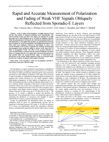
The IEEE Transactions on Antennas and Propagation have recently accepted new research by Chris Deacon G4IFX, Ben Witvliet PE5B, Simon Steendam, and Cathryn Mitchell M0IBG entitled Rapid and Accurate Measurement of Polarization and Fading of Weak VHF Signals Obliquely Reflected from Sporadic-E Layers. This research uses signals produced by a network of 6 meter amateur radio beacons across Europe. Abstract: "In the E-region of the ionosphere, at heights between 90 and 130 km, thin patches of enhanced ionization occur intermittently. The electron density in these sporadic-E (Es) clouds can sometimes be so high that radio waves with frequencies up to 150 MHz are obliquely reflected. While this phenomenon is well known, the reflection mechanism itself is not well understood. To investigate this question, an experimental system has been developed for accurate polarimetric and fading measurements of 50 MHz radio waves obliquely reflected by mid-latitude Es layers. The overall sensitivity of the system is optimized by reducing environmental electromagnetic noise, giving the ability to observe weak, short-lived 50 MHz Es propagation events. The effect of the ground reflection on observed polarization is analyzed and the induced amplitude and phase biases are compensated for. It is found that accurate measurements are only possible below the pseudo-Brewster angle. To demonstrate the effectiveness of the system, initial empirical results are presented which provide clear evidence of magneto-ionic double refraction." A preprint of the research article is available from the University of Bath Website.
Welcome to the HamSCI community! We are a group of amateur radio operators and scientists working together to study the ionosphere and further the amateur radio hobby. If you are completely new to amateur radio and ionospheric science, take a look at the ARRL's What is Amateur Radio page. That is a great place to learn how to get your amateur radio license and learn the basics for participating in the HamSCI community.
HamSCI consists of many different types of projects accessible to a variety of skill levels. Some are more science focused, some are more engineering focused, and some are more focused on the amateur radio hobby. The best way to get involved is to join some of the mailing lists, participate in the telecons, come to the annual HamSCI workshop. You will meet other people in the HamSCI community that can help you to find a project that best matches your interests and skill level. Have a question? E-mail Nathaniel W2NAF at [email protected].
HamSCI Google Group
Participate in the HamSCI Community by joining the HamSCI Google Group. The HamSCI Google Group is an e-mail discussion forum to facilitate communication between hams, the professional space and atmospheric science communities, and anyone else interested. When requesting to join, please include some information about who you are and why you would like to join. If you do not include information on why you would like to join, your request will likely be rejected. Participation is governed by the HamSCI Community Participation Guidelines. This group is moderated by Nathaniel Frissell W2NAF, Kristina Collins KD8OXT, and David Kazdan AD8Y.
If your interest lies with the Personal Space Weather Station, consider joining the HamSCI-psws Google Group. Discussions are welcome on all aspects of the PSWS, including the Grape Doppler receivers, WSPRDaemon SDRs, TAPR/HamSCI Ground Magnetometer, VLF receiving system and the WSPRSonde transmitter network.
TangerineSDR TAPR Listserv
Tucson Amateur Packet Radio (TAPR) is an amateur radio organization dedicated to electrical engineering. TAPR has teamed up with HamSCI to design and build portions of the HamSCI Personal Space Weather Station, including new software defined radios (SDRs), as well as a ground magnetometer system. If you want to be a part of TAPR's SDR and ground magnetometer engineering work, you should join the TangerineSDR listserv by visiting https://tangerinesdr.com/. The TangerineSDR listserv is administered by TAPR and is more engineering focused than the HamSCI Google Group.
HamSCI Weekly Telecons
There are currently three regularly scheduled telecons which support HamSCI's work. All are open to the public, please see the calendar below to confirm teleconference times and view conference call connection information.
TAPR-HamSCI Technical Session: Weekly telecon, hosted on Mondays at 9 PM Eastern (Tuesday 0100z) by TAPR and The University of Scranton to support collaborative HamSCI-TAPR projects.
HamSCI PSWS Operations: Weekly telecon, Thursdays at 10 AM Eastern (1400z), hosted jointly by the University of Scranton, Case Western Reserve University and the University of Alabama. The telecon's primary focus is growing and maintaining the PSWS network, along with management of the collected data.
HamSCIence Telecon: Second Thursday of each month during the academic year at 4 PM Eastern (2000z) to discuss science topics relevant to HamSCI's research efforts. Participants and presenters come from various backgrounds: Professional researchers, academics, students, citizen scientist volunteers. Listen in, ask questions, contact HamSCI if you have a topic you'd like to present.
HamSCI is interested in the effects of the eclipse on signal amplitude as well as Doppler shift. Receivers show this data on an S-meter or Received Signal Strength Indicator (RSSI). This figure shows the effect of the 2017 North American eclipse on a 1350 km path from WWV in Colorado to a receiving station in South Texas. The upper plot is the S-meter voltage from an Icom receiver tuned to 5 MHz WWV and the lower plot is the peak amplitude of the audio output voltage from a 60 kHz WWVB receiver that was not using an Automatic Gain Control (AGC). The effect of the eclipse was to enhance signal strength over this path for both signals by 10 dB. This improvement in propagation was half of the difference in dB between normal day time level and the night time level visible on the far left side of the graph. Signal strength began to increase about an hour before, peaked at local totality, and returned to normal day time propagation over the hour afterwards. The entire path was completely south of the path of totality so it is not necessary for the stations to be directly in or on opposite sides of the path to get measurable results.
Three methods are described for obtaining amplitude data: manually reading the S-meter during the most active local time of the eclipse, setting up a receiver so the audio output voltage amplitude faithfully represents the RF input voltage (WWVB data in the graph) to calibrate the amplitude in the .wav file record, and recording the receiver’s S-meter or RSSI voltage (WWV data in the graph).
Manual Amplitude Record
This is the simplest method of reporting amplitude data for receivers that have an S-meter or RSSI display. Simply write down the average S-meter indication every 10 minutes or so for two hours on either side of maximum totality at your location. You can expect variations as much as 10 dB over a span of seconds from normal fading effects so try to estimate the reading in the middle of the fluctuations for each measurement. Record the UTC time each measurement was taken. While this is the simplest method, it does require you to be present at the radio to periodically read the S-meter during the active part of the eclipse.
S-meters are usually set up with S1 as the lowest reading and increase to S9 at center scale. S9 is historically defined as 50 microvolts into 50 ohms (-73 dBm) and each S unit below S9 represents half of the preceding voltage, or 6 dB per S unit. The markings above S9 are dB’s above S9 and usually have calibration markings at 10 dB increments. If the signal level is below S9, report it as the average of what you see. Example: S8.5. If above, report it as the number of dB’s above S9. Example: S9 plus 15 dB. Some receivers offer the option of expressing RSSI in units of power (dBm). If your receiver has this capability the dBm format is preferred.
Calibrate Audio Output for the .wav File Record
In order to extract accurate amplitude data from a .wav recording of the audio output, the receiver’s AGC (Automatic Gain Control) or AVC (Automatic Volume Control) must be disabled. Otherwise the audio level will be nearly a constant level regardless of the signal strength. Once the AGC is turned OFF the receiver’s RF gain control must be set so that the audio level gives measurable amplitudes that never go full scale, clip, or limit. This will require preliminary testing to be sure the maximum signal strength does not overdrive the sound card input. Here is a method to set up the receiver:
1.With AGC enabled, set up the radio to produce the 1000 Hz tone in USB mode by tuning the radio 1 kHz below the carrier frequency (e.g., 9.999 MHz for a 10 MHz carrier).
2. Set the receiver volume control for a comfortable listening level using the radio’s normal speaker or headphones. It should be loud enough to be above the no-signal receiver noise but not so lout that it causes distortion.
3. Set the recording level in Audacity to get approximately 1/4-1/2 full scale recording level, or at the level that leaves about 6 dB to 10 dB of headroom below full scale.
4. Turn the receiver AGC OFF.
5. Use the RF gain control to set the audio output to the same level as with the AGC ON.
6. Make a day-long recording and examine the record. If the levels reached full scale at any time during the recording, reduce the RF gain control and try again. The idea is to have enough RF gain get measurable signal levels even during the weakest part of the day but not so much that the amplitude at the strongest part of the day hits or flattops at full scale.
7. Once the RF gain is set it must not be changed while recording eclipse data.
Record S-Meter or RSSI Voltage
This is the method used to produce the above data record from WWV and WWVB. It has the advantage of being able to acquire unattended amplitude data and does not require disabling the receiver AGC. Not all receivers port the RSSI voltage externally but some modern radios do. For example the Icom R-8600 receiver and IC-7610 transceiver have a METER output on the rear panel that can be used to record a received signal strength voltage. Consult the operating manual on your radio to see if it has this capability. An AGC response of SLOW is preferred to average out short term amplitude fluctuations. You will need a digitizer capable of responding to a DC voltage. The low frequency roll off in a computer sound card precludes use of a .wav recording. A National Instruments USB-6009 along with National Instruments Signal Express software was used to acquire and display the data in the above figure.
"The question was asked: why do we see sporadic-E like propagation in November and December, when many of the variables like UV radiation and solar exposure are at a minimum, unlike the very active sporadic-E summer months? Much like it was shown that North Atlantic transatlantic 6m propagation during the summer was made more possible by strategically placed weather storm systems, it looks like a similar effect with very strong jet stream boundaries also affect sporadic-e like communications during the winter months. This citizen science study is another example how amateur radio can contribute to science, and illustrates the great potentials for studies using ham radio data. We have many amateur radio stations on the air, using modes like FT8 which make contacts on propagation paths that we thought were previously impossible."
The procedure page is up for December 2020 Eclipse Festival of Frequency Measurement is up! There will be 24-hour practice run on December 5. The main data recording will run from December 9-16.
Chamando todas as estações: Junte-se a nós para no
Festival Eclipse de Medição de Frequência
De 09 de dezembro de 2020 à 16 de dezembro de 2020 2359 UTC
Introdução
Alterações na densidade de elétrons ionosféricos causadas pelo clima espacial e mudanças solares diurnas são conhecidas por causar alterações Doppler nos caminhos/percusos dos raios HF. Por exemplo, consulte a Figura 7 em Boitman et al., 1999. A primeira tentativa do HamSCI de medir essas mudanças Doppler foi durante o eclipse solar total em agosto de 2017. Como parte do WWV centennial, 50 estações coletaram dados de deslocamento Doppler para o Festival de Medição de Freqüência original, demonstrando o valor da participação voluntária na coleta desses dados. Durante o Festival Eclipe de junho de 2020, recrutamos participantes de todo o mundo e experimentamos diferentes protocolos de coleta de dados. Neste inverno, solicitamos que todas as estações de rádio amador, ouvintes de ondas curtas e outros capazes de fazer medições de frequência de alta qualidade HF nos ajudem a coletar dados de frequência para o eclipse total de 14 de dezembro.
Como os caminhos de propagação de estações de tempo padrão (Time standard stations) de ondas curtas variam em um período tempo no calendário?
Quais propriedades da ionosfera somos capazes de medir, observando a variação nesses caminhos de propagação de HF?
Que efeito o eclipse terá sobre esses caminhos de propagação?
Como as várias técnicas de medição para entender a variação do caminho se comparam?
Existe interesse voluntário na coleta de dados em regiões próximas à totalidade deste eclipse ?
Objetivos
Promover a prática internacional de trabalho com cientistas cidadãos em todo o mundo.
Medir as mudanças Doppler causadas pelos efeitos do clima espacial na ionosfera.
Utilizar um protocolo específico de medição disponível para operadores de rádio amadores e outros cientistas cidadãos.
Agenda
Prática de execução:
21 de novembro de 2020, 0000 - 2359 UTC;
4 de dezembro de 2020, 0000 - 2359 UTC.
Início da gravação de dados:
9 de dezembro de 2020, 0000 UTC
Fim da gravação de dados:
16 de dezembro de 2020, 2359 UTC
Comece as medições antes da hora de início e termine-as após a hora de término, se possível.
The Beacons
Existem várias estações de tempo padrão (Time standard stations) que podem ser ouvidas na América do Sul. A estação brasileira PPE (10 MHz) será o farol principal para este experimento. Você também pode captar sinais da estação Venezuelana YVTO (5 MHz), da estação Argentina LOL (5, 10 e 15 MHz), WWV, WWVH e BPM. Este experimento usará apenas as transmissões de 10 MHz. Se você não conseguir obter um bom sinal em 10 MHz, grave outra frequência e certifique-se de que o arquivo esteja devidamente identificado. As gravações neste experimento devem mostrar as formações da camada D no nascer do sol local das estações e outros eventos diários da ionosfera, e os efeitos do eclipse. O clima espacial varia de dia para dia e algumas características podem ser proeminentes. Vamos ver o que temos!
Procedimentos
1) Cadastre-se na Lista de Interessados
Preencha a pesquisa aqui para se inscrever na lista de e-mail. Você receberá atualizações e lembretes ocasionais.
2) Prepare seu receptor
Use seu receptor mais estável. Se você tiver um GPSDO ou outro padrão de frequência de precisão, use-o.
Para sintonizar seu rádio:
Sintonize seu rádio (no modo AM) para o sinal da operadora.
Defina o modo do receptor para USB (banda lateral superior). Para uma portadora de 10 MHz, sintonize em 9,999 MHz (9999.000 kHz - veja a imagem) e ouça o 1000 Hz tom de. Esta é a principal coisa que procuraremos analisaremos nos seus dados.
Se você tiver um filtro ajustável em seu receptor, defina-o o mais próximo possível de 2,5 kHz.
Estamos aconselhando a maioria dos participantes a usar uma taxa de amostragem de 8 kHz na seção abaixo. Se o seu rádio for relativamente novo (fabricado após o ano 2000 ou superior), não haverá problema. Se você estiver executando em um rádio mais antigo, neste caso, seus filtros podem não ter um corte nítido o suficiente. (Você pode ver este processo em um vídeo aqui.) Para verificar a largura de banda do filtro em seu receptor:
Sintonize seu rádio (no modo AM) para o sinal da portadora.
Defina o modo do receptor para USB (banda lateral superior). Para uma portadora de 10 MHz, sintonize em 9,999 MHz (9999.000 kHz - veja a imagem) e ouça o 1000 Hz tom de. Sintonize para 9,998 MHz e ouça o tom mais alto de 2000 Hz. Finalmente, sintonize em 9,997 MHz e veja se você ouve um tom de 3000 Hz. Se você não ouvir um sinal forte da portadora, tudo bem - mantenha 8 kHz. Se você ouvir o tom, use 44100 Hz na Etapa 5 abaixo.
Se estiver trabalhando em um idioma diferente do inglês, você pode defini-lo usando Editar> Preferências> Opções de interface.
3) Configure os metadados do Audacity.
Baixe este modelo XML e memorize o diretório em que ele foi salvo: EclipseTags.xml
Em Editar> Metadados, clique em "Carregar" e selecione o arquivo e, em seguida, edite-o de acordo com a sua estação. (Você também pode adicionar metadados manualmente usando a lista abaixo.)
No Audacity, vá em Edit> Metadata e preencha os seguintes campos de metadados:
Em Artist Name/Nome do Artista, coloque seu indicativo. (Se você é um ouvinte de ondas curtas e não um radioamador, use seu nome ou indicativo SWL.)
No Album title/Título do álbum, coloque "Eclipse de dezembro de 2020".
Em Year/Ano, 2020.
Em Genre/Gênero, coloque o modelo do seu rádio.
Adicione e preencha os seguintes campos de metadados.
Endereço de e-mail
Rig
Antena
Placa de som
Frequência
AGC (ligado ou desligado)
Latitude (use decimais, não minutos e segundos!)
Longitude
Elevação (m)
Fuso horário (exemplo de formato: UTC-03: 00)
Quadrado da grade
País
IMPORTANTE:Se você tem vários rádios coletando dados simultaneamente sob um único indicativo, adicione um hífen e o número da estação para cada estação com o mesmo indicativo. Por exemplo, se a estação W8EDU está executando a coleta de dados simultaneamente em um rádio Flex e um rádio Icom, eles devem marcar um como W8EDU-1 e o outro como W8EDU-2, incluir um comentário nos metadados para cada estação explicando que o operador realizou coletas de várias estações e certifique-se de que os metadados estão corretos e completos. Isso tornará muito mais fácil classificar os dados do experimento durante a fase de análise.
Clique em "Salvar" e salve o arquivo XML, depois clique em "Definir padrão".
Marque a caixa que diz "Não mostrar isso ao exportar áudio" e, em seguida, clique em "OK".
4) Defina as preferências de gravação.
Abra a guia Gravação no menu Preferências (Editar> Preferências> Gravação). Desmarque "Overdub: Reproduzir outras faixas enquanto grava" e marque "Gravar sempre em uma nova faixa".
Em "Nomear novas faixas", digite seu indicativo, um único sublinhado e a letra correspondente ao seu fuso horário nesta lista: [https://en.wikipedia.org/wiki/List_of_military_time_zones]
Por exemplo, a estação W8EDU está no horário de verão do leste (UTC - 05:00), que corresponde à letra R, portanto, o nome correto da faixa customizada é "W8EDU_R_". (Se você estiver em um fuso horário fracionário, use a letra J.)
Certifique-se de que as caixas para "Nome personalizado", "Hora do sistema" e “Hora do sistema”, também estejam marcadas. Quando terminar, a janela deve ser semelhante a esta:
Qualidade
Em Qualidade, definir a taxa de amostragem padrão para 8000 Hz e o formato de amostragem para 16 bits. A não ser que o seu receptor necessidade de taxas altas de amostragens, como descrito anteriormente
Vá para "Dispositivos" no menu Preferências e certifique-se de que está gravando do seu rádio, ao invés do microfone do seu computador ou outra fonte.
5) Defina as configurações de gravação e faça um teste de gravação.
Defina sua gravação como Mono (1 canal) no menu superior, no meio da barra de ferramentas superior.
Caso não tenha definido os padrões de qualidade no tópico anterior para 8000 Hz, defina manualmente este valor na barra de ferramentas superior.
Defina sua entrada de áudio para a placa de som conectada do seu rádio. Os nomes dos dispositivos variam. Você pode ter que realizar alguns testes para certificar-se de que a fonte de áudio da qual você está gravando é a correta.
Aperte o botão Gravar ⬤; você deve ver a primeira faixa começar a gravar, com o nome da faixa e tag de data / hora corretos. Se o nome da faixa não estiver correto, tente reiniciar o Audacity e gravar novamente.
Pressione parar ⏹️ e grave ⬤ novamente. Desta vez, você deve ver uma segunda faixa aparecer. O nome de cada faixa corresponderá ao seu horário de início.
Observe o "Espaço em disco restante para gravação" na parte inferior da tela. Uma semana de gravação dura 168 horas, portanto, pode ser necessário pausar e reiniciar a coleta de dados durante o experimento. A estimativa também pode não ser totalmente precisa. Verifique a documentação do Audacity sobre a duração da gravação aqui.
6) Salve o projeto.
Certifique-se de parar a gravação antes de continuar.
Salve o projeto (Arquivo> Salvar Projeto). Isso permitirá que o computador mantenha suas configurações. Você pode ver uma janela perguntando se você deseja salvar o projeto mesmo que ele não contenha faixas: clique em OK.
7) Certifique-se de que seus arquivos WAV foram salvos corretamente.
Crie um diretório para salvar seus arquivos de acordo com a seguinte convenção: "<Callsign> _Eclipse_Dec2020". Por exemplo: W8EDU_Eclipse_Dec2020. (Se você estiver executando a coleta de dados simultânea em vários rádios, use o identificador hifenizado descrito na Etapa 3.)
Vá para Arquivo> Exportar> Exportar Vários. Selecione o diretório no qual deseja salvar seus arquivos. Em "Name Files", certifique-se de que a opção "Usando Rótulo / Nome da faixa" está selecionada.
Clique em “Exportar”. Você deve obter uma caixa de diálogo confirmando que cada faixa foi salva em seu próprio arquivo WAV.
Quando terminar, você pode excluir suas trilhas de teste clicando no X no canto superior esquerdo da trilha.
Ao abrir o diretório, você deve ver os metadados do artista e do álbum.
Você deve registrar seus dados em uma unidade de disco que tenha pelo menos 10 GB de espaço livre. Se você estiver executando o Windows, navegue até o diretório de dados e ative a compactação: Propriedades -> Geral -> Avançado -> Compactar conteúdo para economizar espaço em disco. (Veja a captura de tela abaixo).
Agora você está pronto para coletar dados! Se você precisar reiniciar a coleta de dados a qualquer momento, aperte o botão para parar a gravação e repita a Etapa 7 acima.
Assim que estiver tudo pronto, sua configuração deve ser semelhante a:
3) Colete os dados
A coleta de dados ocorre de 9 a 16 de dezembro. Haverá também duas práticas mão na massa: 15 de novembro e 5 de dezembro. Durante esse tempo, deixe o seu rádio ligado, verifique-o periodicamente e certifique-se de que o computador não seja desligado por uma atualização automática.
É altamente recomendável registrar alguns dias de dados de teste antes do início do experimento para garantir que você não tenha problemas com o computador. Após a conclusão, antes de enviar, selecione o arquivo / diretório a ser carregado, clique com o botão direito sobre ele e selecione Enviar para pasta compactada (zipada). Isso é o que você deve carregar.
Se você deseja incluir a documentação de sua estação, notas sobre observações, fotos do experimento ou eclipse, etc., inclua-os na pasta compactada com seus dados. A menos que você observe o contrário, podemos usar suas fotos, com atribuição, em materiais futuras da HamSCI.
4) Preencher a pesquisa de coleta de dados e fazer o upload dos dados via Box.
R: Esses dados serão analisados por membros da organização HamSCI. Os dados e resultados serão tornados públicos, como fizemos para o Festival de Medição de Freqüências original.
P: Não estou no caminho da totalidade. Ainda posso participar?
R: Claro, comcerteza. A coleta de dados de estações amplamente dispersas nos permite examinar as flutuações ionosféricas em uma variedade de escalas. Nosso objetivo é obter estações em todos os continentes.
Onde quer que você esteja, no entanto, a melhor abordagem é fazer com que um ou dois amigos com estações próximas participem, para confirmar que as flutuações em seus dados são de natureza geofísica.
P: Perdi a atividade de prática. Ainda posso participar?
R: Sim! Entre em contato por e-mail se tiver dúvidas.
P: Se eu estiver tendo problemas para fazer a coleta de dados funcionar, vocês podem me ajudar?
R: Sim. Envie mail para [email protected] e nós o ajudaremos a configurar o seu rádio.
P: Posso usar um programa diferente do Audacity para fazer minhas medições?
R: Sim, mas não podemos fornecer assistência para outros programas. Mas também gostamos do Spectrum Lab.
P: Por que vocês pararam de usar o fldigi?
R: Usamos o modo de análise de frequência do fldigi em experimentos anteriores, mas decidimos coletar dados brutos para permitir a captura de informações da banda lateral e da portadora.
P: Como posso verificar os metadados em meus arquivos WAV?
R: A maioria das ferramentas de metadados não mostra os campos fora do padrão que adicionamos, mas você pode usar mediainfo se quiser vê-los. Ele também tem uma interface de linha de comando agradável.
P: Por que vocês desejam coletar uma semana inteira de dados? O eclipse não dura apenas algumas horas?
R: Precisamos coletar dados de controle, preferencialmente de um dia com condições ionosféricas que sejam tão semelhantes quanto possível às condições no dia do eclipse. A coleta de uma semana inteira de dados nos dá algumas opções para essa comparação. Também nos dá uma boa visão das flutuações diárias.
P: Você ainda pode usar meus dados se eu não conseguir registrar o período inteiro?
R: Quantomais dados, melhor. Mas se você precisar levar seu rádio de volta para parte do evento (por exemplo, para operar uma rede de tráfego) ou experimentar uma interrupção de dados, ainda estamos interessados em seus dados. Apenas certifique-se de parar a gravação antes de sintonizar novamente seu rádio, sintonize de volta para 9,999 MHz antes de ligá-lo novamente quando estiver pronto para retomar a coleta de dados e deixe-nos uma nota quando enviá-lo.
P: Você aceitará outras formas de dados?
R: Sim, embora não possamos garantir que seremos capazes de usá-los.
P: Consigo configurar uma estação para coletar dados de longo prazo. Você estaria interessado nisso?
R: Sim! Envie email para[email protected] para uma discussão mais detalhada.
P: Vou receber um cartão QSL?
R: Claro! Os certificados do Eclipse Festival serão enviados a todos os participantes na conclusão da análise.
Llamado a todas las radioaficionados. Nos unimos para
El Festival Eclipse de Medición de Frecuencia de Diciembre 2020
9 de diciembre 2020 al 16 de diciembre 2359 UTC
Introducción
Los cambios en la densidad de electrones ionosférico causado por el clima espacial y los cambios diurnos del sol pueden causar desplazamientos Doppler en los trayectos de propagación HF. Por ejemplo, vea la figura 7 en Boitman Et al.,1999. El primer intento a medir eses desplazamientos Doppler de HamSCI fue durante el eclipse solar total en Agosto 2017. Planeamos medidas cuidadosas durante el eclipse total de 2024. Como parte del centenario de WWV, 50 radioaficionados recogido datos sobre los desplazamientos Doppler para Festival de Medición de Frecuencia, demostrando el valor de la recolección voluntaria de datos. Durante el Festival Eclipse de junio 2020, solicitamos la ayuda de los participantes del todo el mundo y experimentamos con diferentes protocolos para la recopilación de datos. Este invierno, solicitamos que todas las radioaficionados, radioescuchas de onda corta, y otras que pueden medir las frecuencias HF con precisión ayúdanos a recoger datos de la frecuencia para el eclipse total en el 14 de Diciembre.
¿Cómo varían los caminos de propagación de los estaciones de tiempo de onda corta estándar durante un día completo de calendario?
¿Qué propiedades del ionosfera podemos medir observando los cambios en los caminos de propagación HF?
¿Que efecto va a tener el eclipse en estos caminos de propagación?
¿Cómo se comparan técnicas de medir diferentes para comprender los caminos de propagación?
¿Hay interesa voluntario a recoger datos cerca al camino de la totalidad de este eclipse?
Objetivos
Promover la buena voluntad internacional trabajando con científicos amateur desde el mundo.
Medir los desplazamientos Doppler causado por el clima espacial en la ionosfera.
Utilizar un protocolo de medida específico disponible a las radioaficionados y otros científicos amateur.
Horas de Operación
días de práctica: 21 Noviembre 2020, 0000 - 2359 UTC, 4 de diciembre de 2020, 0000 - 2359 UTC
Recopilación de datos empeza al 9 diciembre de 2020, 0000 UTC
Recopilación de datos termina al 16 diciembre de 2020, 2359 UTC
Por favor, si es posible, comenzar las mediciones antes de la hora de empezar y terminar las mediciones después de la hora de terminar.
Las Radiobalizas
Hay muchas radiobalizas que se pueden escuchar en América del Sur. La estación brasileña PPE (10 MHz) será la radiobaliza principal para este experimento.También puede recibir señales de radio de la estación venezolana YVTO (5 MHz), la estación argentina LOL (5, 10, y 15 MHz), WWV, WWVH, y BPM. Para este experimento, solo usaremos las transmisiones de 10 MHz. Sí quiere participar pero no puede grabar o obtener una buena señal en 10 MHz, puedes usar la frecuencia que puedes grabar y etiquetar su archivo apropiadamente. Las grabaciones en este experimento muestren formaciones de la capa D al amanecer local de las estaciones y otros eventos diarios de la ionosfera y los efectos del eclipse. El clima espacial varía día a día y algunas características pueden ser prominentes. ¡Vamos a ver lo que obtenemos!
Procedimientos
1) Inscribirse en la lista de intereses
Complete la encuesta aquí para inscribirse en la lista de correo electrónico. Vas a recibir actualizaciones y recordatorios ocasionales.
2) Prepara su receptor
Utiliza tu receptor más estable. Sí tiene un GPSDO o otro estándar de frecuencia de precisión, usarlo..
Para sintonizar su radio:
Sintonice su radio (en modo AM) a la onda portadora.
Establezca el modo de su receptor en USB (banda lateral superior). Para 10 MHz, sintonice a 9.999 MHz y escuche el tono de 1000 Hz. Esto es lo principal que buscaremos cuando analicemos sus datos.
Si tiene un filtro ajustable en su receptor, ajústelo lo más cerca posible de 2,5 kHz.
Aconsejaremos a la mayoría de los participantes que utilicen una frecuencia de muestreo de 8 kHz en la sección de abajo. Si su radio es relativamente nueva (fabricada después del año 2000 aproximadamente), debería estar bien. Si utiliza una radio antigua, es posible que sus filtros no tengan un corte lo suficientemente afilado. (Puede ver este proceso en un video aquí.) Para verificar el ancho de banda del filtro en su receptor:
Sintonice su radio (en modo AM) a la onda portadora.
Establezca el modo de su receptor en USB (banda lateral superior). Para 10 MHz, sintonice a 9,999 MHz y escuche el tono de 1000 Hz. Sintonice hasta 9,998 MHz y escuche al tono más alto en 2000 Hz. Finalmente, sintonice a 9,997 MHz y escucha para un tono de 3000 Hz . Si no escucha una señal de onda portadora fuerte, está bien: quédese a 8 kHz. Si escucha el tono, use 44100 Hz en el Paso 5 a continuación.
3) Prepare su computadora y software
1) Conecte su radio a la tarjeta de sonido de su computadora.
Si está controlando su radio a través de fldigi o flrig, ya sabes cómo hacerlo. Las instrucciones variarán según la radio. Si necesita una tarjeta de sonido USB, recomendamos este: https://www.amazon.com/gp/product/B00IRVQ0F8/ref=ppx_yo_dt_b_asin_title_o03_s00?ie=UTF8&th=1
2) Descarga Audacity.
Audacity es un programa de código abierto bien establecido para la grabación de audio. Puede descargarlo aquí: https://www.audacityteam.org/download/
Si está trabajando en un idioma que no sea inglés, puede configurarlo usando Editar> Preferencias> Interface y selectar a su idioma.
3) Configure los metadatos de Audacity.
Descargue esta plantilla XML y anote el directorio que descarga en: EclipseTags.xml
En Editar> Metadatos, haga clic en "Cargar" y seleccione el archivo. Después, puedes editarlo para que se ajuste a su estación. (También puede agregar metadatos manualmente usando el lista a continuación.)
En Audacity, vaya a Editar> Metadatos y complete los siguientes campos de metadatos:
En Nombre del artista, entra su indicativo. (Si estas un oyente de onda corta y no un aficionado, utilice su nombre).
En Título del álbum, entra "Eclipse de diciembre de 2020".
En Año, entra “2020”.
En Género, entra su modelo de radio.
Agregue y complete los siguientes campos de metadatos. Por favor, escribe estos campos de metadatos en inglés para consistencia de datos.
Dirección de correo electrónico “Email”
modelo de radio “Rig”
Antena “Antenna”
Tarjeta de sonido “Sound Card”
Frecuencia “Frequency”
AGC (activado o desactivado) “AGC”
Latitud (utilice decimales, no minutos y segundos) “Latitude”
Longitud “Longitude”
Elevación (m) “Elevation (m)”
Zona horaria (Ejemplo de formato: UTC-05: 00) “Time Zone”
Cuadrícula Cuadrado “Grid Square”
País “Country”
IMPORTANTE:Si tiene varias radios que recopilan datos simultáneamente con un solo indicativo, agregue un guión y un número de estación para cada estación donde de otra manera usaría el indicativo. Por ejemplo, si la estación W8EDU está grabando la recopilación de datos simultáneamente en una radio Flex y una radio Icom, deben etiquetar una como W8EDU-1 y la otra como W8EDU-2, incluir un comentario en los metadatos para cada estación explicando que el operador grabó varias estaciones y asegúrese de que los metadatos sean correctos y estén completos. Esto hará que sea mucho más fácil clasificar los datos del experimento durante la fase de análisis.
Haga clic en "Guardar" y guarda el archivo XML. Después haga clic en "Establecer Valores Predeterminados".
Marque la casilla que dice "No mostrar esta advertencia exportar audio", y haga clic en "Aceptar".
4) Establecer preferencias de grabación.
Abra la pestaña Grabación en el menú Preferencias (Editar> Preferencias> Grabación). Desmarca "Reproducir otras pistas mientras se graba" y marca "Grabar en una pista nueva" y "Detectar pérdidas".
En "Nombre de nuevas pistas de grabacion", escribe tu indicativo, luego un guión bajo y luego la letra correspondiente a tu zona horaria en esta lista: [https://en.wikipedia.org/wiki/List_of_military_time_zones]
Por ejemplo, la estación W8EDU está en horario de verano del este (UTC - 05:00), que corresponde a la letra R, por lo que el nombre correcto de la pista personalizada es "W8EDU_R_". (Si se encuentra en una zona horaria fraccionaria, use la letra J.)
Asegúrese de que las casillas de "Fecha" y "Hora" también estén marcadas. Cuando estas terminado, la ventana debería verse así:
Vaya a “Calidad” en el menú Preferencias y marca “Formato de muestra predeterminado” a “16 bits” y marque “Frecuencia de muestreo predeterminada” a 8000 Hz (a menos que su radio necesitas una tasa más alta como describió en el paso 2 anterior)
Vaya a "Dispositivos" en el menú Preferencias y asegúrese de que está grabando desde su radio, en lugar del micrófono de su computadora.
5) Configure los ajustes de grabación y grabe una grabación de prueba.
Configure su grabación en 1 canal de grabación (Mono) en el menú en la mitad superior de la pantalla.
Asegúrese de que la tasa de su proyecto es 8000 Hz desde el menú en la esquina inferior izquierda de la pantalla.
Configure su entrada de audio a la tarjeta de sonido conectada a su radio. Los nombres de los dispositivos variarán. Puede que tenga que experimentar para asegurarse de que la fuente desde la que está grabando sea la correcta.
Haga clic en el botón Grabar ⬤; debería ver la primera pista de inicio de grabación con el nombre de pista y la marca de tiempo correctos.
Si el nombre de la pista no es correcto, reiniciar su computadora y grabar otra vez.
Presiona detener ⏹️, luego graba ⬤ otra vez. Esta vez, debería ver aparecer una segunda pista. El nombre de cada pista corresponderá a su hora de inicio.
Tenga en cuenta el “Espacio en disco disponible para grabaciones” en la parte inferior de la pantalla. Una semana de grabación es 168 horas, así que es posible que debes necesitar pausar y reiniciar la recopilación de datos durante el experimento. Es posible que la estimación no sea del todo precisa. Consulte la documentación de Audacity sobre la duración de la grabación aquí.
6) Guardar el proyecto.
Asegúrese de detener ⏹️ la grabación antes de continuar.
Guarde el proyecto (Archivo> Guardar Proyecto). Esto permitirá que la computadora guarde su configuración. Es posible que vea una ventana que le pregunte si desea guardar el proyecto aunque no tenga pistas: haga clic en Aceptar.
7) Verifique que sus archivos WAV se guarden correctamente.
Cree un directorio para guardar sus archivos de acuerdo con la siguiente convención: "<Callsign> _Eclipse_Dec2020". Por ejemplo: W8EDU_Eclipse_Dec2020. (Si está grabando datos simultánea en varias radios, use el identificador con guión descrito en el Paso 3).
Vaya a Archivo> Exportar> Exportar múltiple. Seleccione el directorio en el que desea guardar sus archivos. En "Archivos de nombre", asegúrese de que la opción "Usar nombre de etiqueta o pista" esté seleccionada.
Haga clic en "Exportar". Debería aparecer un cuadro de diálogo que confirme que cada pista se ha guardado en su propio archivo WAV.
Cuando estás terminado, puede eliminar sus pistas de prueba haciendo clic en la X en la esquina superior izquierda de la pista.
Cuando abra el directorio, debería ver el artista y los metadatos del álbum.
Debe grabar sus datos en un disco duro que tenga al menos 10 GB de espacio libre.
¡Ahora debería estar listo para recopilar datos! Si necesita reiniciar la recopilación de datos en cualquier momento, presione el botón de detener la grabación y repita el paso 7 anterior.
Cuando estas todo listo, su configuración debería verse así:
3) Recopilar los datos
La recopilación de datos se realiza del 9 al 16 de diciembre. También hay dos prácticas: el 15 de noviembre y el 5 de diciembre. Durante este tiempo, deje su radio sola y asegúrese de que su computadora no esté apegada para una actualización automática.
Recomendamos encarecidamente registrar los datos de práctica de unos días antes de que comience el experimento para asegurarse que no tiene problemas con su computadora. Después de completar, pero antes de cargar, seleccione el archivo / directorio que se cargará, haga clic derecho sobre él y seleccione Enviar a carpeta comprimida (zip).
Si quieres incluir documentación de su estación, notas sobre observaciones, fotos del experimento o eclipse, etc., inclúyase en la carpeta comprimida con sus datos. A menos que indique lo contrario, podemos utilizar sus fotos, con atribución, en futuros materiales de HamSCI.
4) Complete la encuesta de recopilación de datos y cargue los datos a través de Box.
Completa la encuesta de recopilación de datos aquí.
R: Esta información será analizada por miembros de la organización HamSCI. Los datos y resultados se harán públicos, como lo hicimos para el Festival original de Medición de Frecuencia
P: No estoy en el camino de la totalidad. ¿Todavía puedo participar?
R: Por supuesto, sí. La colección de datos de radioaficionados muy dispersos nos permite examinar las fluctuaciones ionosféricas en una variedad de escalas. Nuestro objetivo es conseguir estaciones en todos los continentes.
Independientemente de dónde se encuentre, el mejor enfoque es conseguir que uno o dos amigos radioaficionados que están cerca de ti participen para confirmar que las fluctuaciones en sus datos son de naturaleza geofísica.
P: Me perdí el día de control.. ¿Todavía puedo participar?
R:¡Por supuesto, sí! Envíenos un correo electrónico si tienes preguntas.
P: Si tengo problemas para que la recopilación de datos trabaje, ¿pueden ayudarme?
R: Sí, envíenos un correo electrónico a [email protected] y podemos asistir a configurar su radio.
P: ¿Puedo usar un programa que no sea Audacity para realizar las mediciones?
R: Sí, pero no podemos ayudar para otros programas, aunque también nos gusta Spectrum Lab.
P: ¿Por qué dejó de usar fldigi?
R: Hemos utilizado el modo de análisis de frecuencia fldigi en experimentos anteriores, pero decidimos recopilar datos sin procesar para este experimento porque nos permitirá recopilar información de banda lateral y de portadora.
P: ¿Cómo puedo verificar los metadatos en mis archivos WAV?
R: La mayoría de los campos de metadatos que agregamos no aparecen en en la mayoría de los programas. Pero, puede usar “mediainfo” si quieres verlos. También tiene una bonita interfaz de línea de comandos.
P: ¿Por qué quieres que nosotros recopilar una semana completa de datos? ¿No dura el eclipse solo unas pocas horas?
R: Necesitamos recopilar datos de control, idealmente de un día con condiciones ionosféricas que sean lo más similares que posible a las condiciones del día del eclipse. La recopilación de una semana completa de datos nos da algunas opciones para esa comparación. También nos da una buena visión de las fluctuaciones diarias.
P: ¿Puedes usar mis datos si no puedo grabar para el periodo completo?
R: Más datos es mejor que menos, pero si necesita usar su radio durante el el evento para dos o tres horas, todavía tenemos interesa entre sus datos. Solo asegúrate de salir del modo de análisis de frecuencia antes de utilizando su radio, y sintoniza su radio a 9,999 MHz antes de continuar recolectando más datos y deje una nota cuando lo sube.
P: ¿Vas a aceptar otras formas de datos?
R: Sí, aunque no podemos garantizar que podamos usarlo.
P: Puedo establecer un estación para recoger datos a largo plazo. ¿Estaría interesado en eso?
R: ¡Por supuesto, Sí! Envíenos un correo electrónico a [email protected] para discutir con más detalle.
P: ¿Voy a recibir una tarjeta QSL?
R: ¡Por Supuesto! El festival del Eclipse va a mandar tarjetas a todas las personas que participan cuando el experimento termina.
The ARRL Frequency Measurement Test (FMT) is a bi-annual event that has its roots back to 1931! Back then, it was needed to ensure that Official Observers (OOs) could correctly callibrate their radios for monitoring and policing purposes. The FMT is still quite relevant today, but for different reasons. Today, the most significant source of error on a stable recieved signal will be due to ionospheric variability. Therefore, making frequency measurements is of great interest to the HamSCI community. These types of measurements are some of the inspiration for the HamSCI Festival of Frequency campaigns and the Low-Cost Personal Space Weather Station. The FMT is a great way to get started in learning how to take precision ionsopheric measurements. A new Frequency Measurement Test mode added to the free FLDigi program makes it even easier to participate. You can now download an article entitled "Using Fldigi for the ARRL Frequency Measuring Test (FMT)" by Bob Howard, VE3YX, to help get you started. The next FMT will be November 13, 2020 from 0200Z-0524Z. . Practice FMT sessions are being conducted by the fmt-nuts group as posted on their home page at https://groups.io/g/fmt-nuts. . Practice FMT sessions are being conducted by the fmt-nuts group as posted on their home page at https://groups.io/g/fmt-nuts. More details are available at https://fmt.arrl.org/ and in the November 2020 QST article by Ward Silver, N0AX. Thank you to FLDigi author Dave Freese W1HJK for his hard work in developing FLDigi and this new mode!
Ash Chaabane, 3V/KF5EYY, reports that a new Reverse Beacon Network (reversebeacon.net) node has been successfully installed in Tunisia. There will soon be an Algerian and Libyan node when logistics permit. The Tunisian node consists of a DX Engineering ARAV4-1P active vertical antenna (see the photo, contributed by Ash), a Red Pitaya 122-16 SDR, and CW Skimmer software by VE3NEA. You can see the stations reported on several bands by the new node at https://dxcluster.ha8tks.hu/azimuthal_map/index.php?c=3V/KF5EYY&t=de. This node was part of a Yasme Foundation (yasme.org) project to install more RBN nodes in out-of-the-way places not currently home to a receiver. The project aims to support both the amateur radio community and spaceweather/geophysics research community with propagation information from around the world and raise awareness of amateur radio's long-standing history of supporting science. Additional nodes are planned for the Caribbean, South Pacific, and Russia, while other groups are installing nodes in Australia.
Video recordings of the third annual HamSCI Workshop are now available through the Ham Radio 2.0 YouTube Channel. The 2020 HamSCI Workshop for amateur radio operators and professional scientists was held Friday and Saturday, March 20-21, 2020, virtually on Zoom at The University of Scranton. The theme of the workshop was “The Auroral Connection,” and included addresses by guest speakers, poster presentations, and demonstrations of relevant instrumentation and software.
The workshop served as a team meeting for the HamSCI Personal Space Weather Station project, which is a National Science Foundation (NSF) funded project awarded to University of Scranton physics and electrical engineering professor Nathaniel Frissell, W2NAF. The project seeks to harness the power of a network of licensed amateur radio operators to better understand and measure the effects of weather in the upper levels of Earth’s atmosphere, as well as provide new tools to help amateurs understand radio propagation and improve operating. Through the grant, Dr. Frissell, a space physicist, will lead a collaborative team that will develop modular, multi-instrument, ground-based space science observation equipment and data collection and analysis software. The PSWS is led by The Univeristy of Scranton, and includes participation from TAPR, Case Western Reserve University/W8EDU, the University of Alabama, the New Jersey Institute of TechnologyCSTR, MIT Haystack Observatory, Dartmouth College, and the ham radio community at large.
Invited speakers at the workshop included Elizabeth MacDonald, Ph.D., the NASA researcher that founded and leads the Aurorasaurus project. Dr. MacDonald discussed fundamentals of auroral physics, its optical signatures, and the Aurorasaurus citizen science project. James LaBelle, Ph.D., professor of physics and astronomy at Dartmouth University and auroral radio physicist, discussed radio signatures of the aurora, remote sensing using active and passive techniques, and ways the amateur radio/HamSCI community could contribute. David Hallidy, K2DH, a retired microwave engineer who is also a well-known amateur radio operator for his work in auroral mode propagation, discussed his practical experiences of using the aurora for radio communication purposes. Tim Duffy, K3LR, well-known contester and chief executive officer and general manager at DX Engineering gave keynote remarks entitled "Let’s Push the Exploration of the Ionosphere to The Next Level".
Dr. Nathaniel Frissell, W2NAF, The University of Scranton, Chair
Dr. Travis Atkison, The University of Alabama
Dr. Kristina Collins, KD8OXT, Case Western Reserve University, Space Science Institute
Mr. Ed Efchak, WX2R, HamSCI Community
Mr. William Engelke, AB4EJ, The University of Alabama
Dr. Phil Erickson, W1PJE, MIT Haystack Observatory
Mr. William Liles, NQ6Z, HamSCI Community
Dr. Hyomin Kim, KD2MCR, New Jersey Institute of Technology
Mr. Gary Mikitin, AF8A, HamSCI Community
Dr. Ethan Miller, K8GU, STR
Dr. Gareth Perry, KD2SAK, New Jersey Institute of Technology
Mr. H. Ward Silver, N0AX, HamSCI Community
Dr. Mary Lou West, KC2NMC, Montclair State University
Dr. Christian Zorman, KF8FPA, Case Western Reserve University
Community Moderators
Dr. Nathaniel Frissell, W2NAF, University of Scranton
Dr. Kristina Collins, KD8OXT, Case Western Reserve University
Dr. David Kazdan, AD8Y, Case Western Reserve University
Activity Coordinators
Gary Mikitin, AF8A, Amateur Radio Community Coordinator
Ed Efchak, WX2R, Public Information Officer
General Membership
Membership is open by joining the HamSCI Google Group, which, as of mid-2026, numbered over 1,500 participants. HamSCI appreciates all of its members, their interest, their efforts and their contributions to HamSCI's mission.
Code is important to our work at all stages, and well-written code might impact both our own accomplishments within teams, as well as how useful our work will be to the world in general. This is true for the Personal Space Weather Station, but also for so many of our projects, academic papers, and more. I therefore propose a regular code review session for the HamSCI community. Meeting and discussing code will help us improve our programming skills individually, and the quality of our work as a community.
Feel free to send along ideas (contact information is below).
When
weekly meetings of 1 hour
You are welcome to come to as many or as few code review meetings as you like.
Time tbd
Where
zoom, tentatively
Who
All experience levels are welcome.
Some help from those with more programming experience would be much appreciated, but those of us know are newer to programming still have a lot to offer and learn from each other!
You don't have to bring code to discuss to the session, though if you've been working on something lately, we'd encourage you to bring it.
No affliation with HamSCI is necessary (though you should come join us, it's fun!).
What code you can bring for discussion
You are welcome to bring code from any HamSCI project, or work that is of interest to the amateur radio or scientific communities and consistent with the objectives of HamSCI. Code in any programming language is welcome.
You must have the right to share and discuss the code you are presenting.
While everyone is welcome to make use of the general concepts and programming techniques discussed in other projects, being part of code review does not grant the other participants rights to the specific software being discussed. Participants agree to not use, distribute, or discuss the sofware in ways not explicitly granted by the code's presenter.
Bringing Code to the Review
First-come first-serve, though people may email me to request to be on the list for discussion
ordering will be at organizers' discretion preference will be given to newer programmers or those who haven't gotten floor time lately
You should have your code and any supporting files ready to share. You should also have prepared a copy of your code that you can share with the participants if necessarily.
You might come with a small number of specific questions you'd like to ask to the group, or you might ask for general feedback on your work.