PSWS VLF Receiver and Magnetometer
PSWS VLF Receiver and Magnetometer
Destination Url
/psws
PSWS VLF Receiver and Magnetometer
/psws
PAGE MOVED: Please visit http://hamsci.org/hamsci2022

This week, many HamSCI members are presenting their research at the American Geophysical Union (AGU) Fall Meeting in New Orleans and Virtually Online. The AGU Fall meeting is one of the largest profession geoscience meetings in the world, and consists of about 24,000 attendees. The scientific program includes sessions pertaining to all areas of geophysics, including space weather, the solar wind, auroral activity, the ionosphere, and the neutral atmosphere. Below is a list of selected presentations and sessions being given by HamSCI members, or of general interest to ham radio operators. The complete scientific program is available here.
Traveling ionospheric disturbances are space weather in nature and cause fluctuations in electron density that can have impacts on HF propagation. Two techniques, GNSS based total electron content (integrated density through the ionosphere and plasmasphere), and incoherent scatter radar (direct altitude profiles of temperature, density, velocity), can provide spatial structure information on these disturbances.
Solar flares cause D region based HF blackouts, but have effects through the ionosphere and neutral atmosphere. September 2017 was characterized by multiple solar flares as well as large geomagnetic storm perturbations. Studying these helps understand the system's response to forcing.
At mid-latitudes over North America, we have known for more than a decade that HF radars (SuperDARN) see almost constant backscatter from small-scale irregularities moving at slow ionospheric speeds. The causes of these irregularities are still under investigation, but they are very useful as a remote diagnostic. This will give updates on progress toward understanding the irregularity origins. Their presence may cause short time period HF propagation path changes.
SNASH was created to act as a surveillance recorder for the December 2021 Eclipse Festival of Frequency Measurement and other citizen science campaigns involving timed audio recording.
https://github.com/Tara162299/SNASH
Metadata template for December 2021 Eclipse Festival: SNASH_dec_2021_eclipse_festival.xml
Download and install from the link above.
1) Make sure Windows is set to use the audio channel from your radio as the default sound input.
2) Open SNASH from your Programs menu.
3) Click "Select Configuration File" and browse to find the .XML file for the experiment you're participating in. (It is included in the zipped folder used for alpha testing, above.)
4) Make sure to fill in all the metadata fields! The following have special instructions:
Also, keep in mind:
Tip: You may want to save a copy of this metadata file and change the default values according to your needs. (This is particularly useful so that you don't have to type in your latitude and longitude every time you want to stop and start the recording...)
Once you're happy with your metadata, select a location for your files to save. Start and stop the recording and confirm that the files (a) are saved in that location, and (b) playable. You can also use mediainfo's command line tool to verify that your metadata is saved properly.
If you run into any issues with this process, please submit them to the Feedback form below. Remember that this piece of software is under test, and we value your feedback.

Our sense of sound can be a powerful tool in exploring and analysing data collected from satellites. But what is the best way to make this data audible? Space science researchers at Imperial College London are asking for input from communities with relevant expertise (including Audio, Citizen Science, Music, Public Engagement, and Science Communication) to help us choose the best method of making Ultra-Low Frequency waves around the Earth audible. Fill out our quick survey telling us which you think sounds best. It shouldn’t take more than 10 minutes. Your valuable feedback and recommendations will help space scientists around the world to improve science communication, public engagement, and citizen science.
If you would like further information please contact Dr Martin Archer, Stephen Hawking Fellow in Space Physics at Imperial College London via [email protected]. Thank you for your help!
You can read the recent article on the WWV/H Scientific Modulation Working Group here: WWV/WWVH Scientific Modulation Working Group | WWVARC
For up-to-date information on the working group, check out the main page here: www.hamsci.org/wwv

Come join HamSCI at its fifth annual workshop March 18-19, 2022 at the U.S. Space and Rocket Center in Huntsville, Alabama. The primary objective of the HamSCI workshop is to bring together the amateur radio community and professional scientists. The theme of the 2022 HamSCI Workshop is The Weather Connection.
This workshop will also serve as a team meeting for the HamSCI Personal Space Weather Station project, a NSF-funded project to develop a citizen science instrument for studying space weather from your backyard. The PSWS is led by the University of Scranton, and includes participation from TAPR, Case Western Reserve University/W8EDU, the University of Alabama, the New Jersey Institute of Technology CSTR, MIT Haystack Observatory, Dartmouth College, and the amateur radio community at large.
The 2022 HamSCI workshop is organized by The University of Scranton in collaboration with The University of Alabama and NASA Marshall Space Flight Center. Support is provided by the National Science Foundation.

Please e-mail [email protected].

The 2022 HamSCI Workshop is organized by The University of Scranton in collaboration with The University of Alabama and NASA Marshall Space Flight Center. Financial support is provided by the United States National Science Foundation through AGS-2152015.
As part of HamSCI Personal Space Weather Station (PSWS) project, magnetometers which measure magnetic field strength and direction, are designed to provide quantitative and qualitative measurements of the geospace environment from the ground for both scientific and operational purposes at a cost that will allow for crowd-sourced data contributions.
The PSWS magnetometers employ a low-cost, commercial off-the-shelf, magneto-inductive sensor technology to record three-axis magnetic field variations with an adequate field resolution of less (or better) than 10 nT at a 1 Hz sample rate. Data from the PSWS network will combine these magnetometer measurements with high frequency (HF, 3-30 MHz) radio observations to monitor large-scale current systems and ionospheric disturbances due to drivers from both space and the atmosphere. A densely-spaced magnetometer array, once established, will demonstrate their space weather monitoring capability to an unprecedented spatial extent.
The primary goals are 1) to provide the general context of geomagnetic activity during the HF experiments proposed in the PSWS project; 2) to estimate ionospheric currents at mid/high latitudes; 3) to measure space weather-related disturbances (dB/dt) at higher latitudes.
HF communication is very much affected by the ionospheric conditions which are inarguably associated with the solar and geomagnetic activity. Magnetic field observations provide critical information about such an interaction (#1). As for #2, the proposed densely-spaced magnetometer network can also provide a complementary data set to help infer ionospheric currents over the entire region where the PSWS is located. At present, ground magnetometers for space research are located primarily near/in the auroral regions. The US government-funded magnetometers are sparsely located across the US at mid latitudes. The HamSCI magnetometer network will help increase the spatial resolution of the magnetic field measurements instead of taking on the existing infrastructure which is designed to provide well-calibrated absolute values of geomagnetic fields.
The higher spatial density is one of the major unique aspects of the PSWS project. Typically, ground magnetic field data are used to infer equivalent current systems (“E x B drift”) in the ionosphere by combining the horizontal fields at multiple locations (e.g. Amm et al., 2002; Kim et al., 2015). At higher latitudes where more geomagnetic L-shells are concentrated, a more densely-spaced sensor network is desired to increase the number of measurement points and thus to avoid interpolations based on an assumption that ionospheric conditions are uniform between the measurement points: we know that this is an oversimplification. While high-latitude (> auroral region), multi-point magnetic fields from a densely-spaced sensor network have reported in a number of papers, mid-latitude observations of geomagnetic fields from a densely-spaced sensor network have never been done.
Space weather-related events (e.g., geomagnetically induced current or GIC, related to dB/dt) are also target observations, especially at high latitudes (e.g., Alaska) as stated in #3. Measurements of dB/dt with a higher spatial resolution have not been conducted as well.
The target specifications and performance level of the magnetometer are: a) time-varying field measurements in three axes; b) less than 10 nT resolution at 1 Hz sample rate; and c) ~50-100 mile spacing.
One can argue that low/mid-performance magnetometers in your backyard may not add any scientific value. The following is the counter-argument:
Amm, O., Engebretson, M. J., Hughes, T., Newitt, L., Viljanen, A., and Watermann, J., A traveling convection vortex event study: Instantaneous ionospheric equivalent currents, estimation of field-aligned currents, and the role of induced currents, J. Geophys. Res., 107( A11), 1334, doi:10.1029/2002JA009472, 2002.
Kim, H., Clauer, C. R., Engebretson, M. J., Matzka, J., Sibeck, D. G., Singer, H. J., Stolle, C., Weimer, D. R., and Xu, Z. (2015), Conjugate observations of traveling convection vortices associated with transient events at the magnetopause. J. Geophys. Res. Space Physics, 120, 2015– 2035. doi: 10.1002/2014JA020743.
Ver. 1.0
David Witten
1. Make sure to set up a Raspberry Pi password
2. Set up system time to UTC
$ sudo raspi-config
3. Install data acquisition software
$ sudo apt-get update
$ sudo apt-get install git
$ git clone https://github.com/wittend/rm3100-runMag
$ cd rm3100-runMag
$ make
If there is an earlier code on the Raspberry Pi:
$ cd rm3100-runMag
$ make clean
$ git pull
$ make
4. Run the software
4.1. For a long-term operation
$ ./runMag -kPS [SITEID*]
OR
$ ./runMag -kS [SITEID*]
(The -P optionn causes the program to print out the initial settings (to the screen) to let you know what settings you have given – mostly for debugging - may be omitted)
*SITEID: Create your own site ID for others to recognize the location of the magnetometer.
This should start the program, putting logged output into file named something like:
../logs/<site ID>-20200623-runmag.log
appears in the logs directory. The program should continue to append to this file until 23:59:59 when the program closes this file and opens a new one, in this case:
../logs//<site ID>-20200624-runmag.log
It then continues to append to this file for the next 24 hours, and repeats this process.
Note: to be paired with a newly assembled sensor assembly (provided by Julius Madey), use the following command:
$ ./runMag -H -M 0x23 -A 10 -c400 -U140 -kPZS <your callsign> &
(for the older sensor, try to use 0x20)
This will NOT show output to the screen. It writes to the logfile.
4.2. For a short-term testing
$ ./runMag or ./runMag -H
This will show the output of the program on the console Without logging to file.
If you want to write to the log file but also view the output:
$ ./runMag -k -S [SITEID].
Then open another terminal window in the same folder and type:
$ tail -n 15 -f logs/[SITEID]-[UTCDATE]-runmag.log.log
This is to read the logfile as it is written. It displays outpout log file as it is wirtten in the window. This will work until the UTC date changes (8:59 pm edt). At this poiint the data will begin to be logged to a new file:
../logs/[SITEID]-[UTCDATE + 1]-runmag.log.log
and the display in the window will just stop. (because the original logfile is not being written to any more).
Another method,
runMag | tee > logs/[SITEID]-[CURRENT UTC TIME]-runmag.log
This version will not roll the log file over at 00 UTC.
4.3. Other options
$ ./runMag -l -Z - b 1
$ ./runMag -Z - b 1 > data.txt :
This Creates and writes output to a file named ‘data.txt’. Will overerite previous file with that name.
$ ./runMag -Z - b 1 >> data.txt:
This Creates or Appends to an existing file named ‘data.txt’. Will not overwrite existing file.
$ ./runMag -Z - b 1 | tee data.txt: This command uses a command line trick to split the output between the storage file ( data.txt ) and the console window Program was launched from.
$ ./runMag -lkS <site id>
This command line will read only the local thermometer chip and then write the results to a file in ./logs/ called something like JennyJump-20200703-runmag.log. Data will be appended to this until 23:23 UTC (should be 08:23 edt for you). At that point that file will be closed, another file will be opened with the name JennyJump-20200704-runmag.log and log entries should be entered into this new file for the next 24 hours. Then the process repeats ad infinitum.
$ tail -f ./logs/jjump01-20210307-runmag.log
To view the contents of the log file that it is writing.
To do this, press enter one time and get your prompt.
Type the command tail -f followed by the name (with path) of the log file that is being written.
This will print each new line written to the logfile to the screen. This will continue until you use CTRL-C or until 00:00:00 UTC, at which time no new lines will be displayed (8:00 pm EST). The reason that the output stops at that time is that runMag has closed the initial log file and opened a new one. To see the new log file being created, reenter the command from before, but increment the date part of the file name by one. For example: tail -f ./logs/jjump01-20210308-runmag.log
5. Power interruption Mitigation
This is based on an assumption that the Raspberry Pi is connected to the internet and has access to internet time and the board is configured to quickly calibrate its internal time using the internet time services (ntp). This is the usual case for properly configured Raspberry-Pi’s.
There are (at least) two situations where time keeping will be degraded.
If network connectivity is lost for some period the measurements recorded are likely to drift in time because the internal clock on Rpi’s is pretty poor and not ordinarily backed up. The system in this case will continue logging data, but the trustworthiness of the timestamps will degrade. The log files may not roll at precisely 23:23 UTC. This is not usually the case for Odroid boards which do provide a battery backed real time clock.
The second situation is one where the Raspberry Pi loses its main power or the program is manually stopped. If the program is restarted within the same UTC DAY using the same parameters that were used before, logging will continue to the same output file as before. The only consequence will be that there will be a gap in the data equivalent to the down time. But the time stamps should be reasonably coherent across the gap in the samples.
The real solution for deploying these devices for long-term evaluation with limited supervision is to load a software package such as GPSd and a simple but reliable GPS module such as the Adafruit Ultimate GPS hat plus some sort of UPS supply designed for Pi or Odroid boards. I have these Items available. I can provide them if desired.
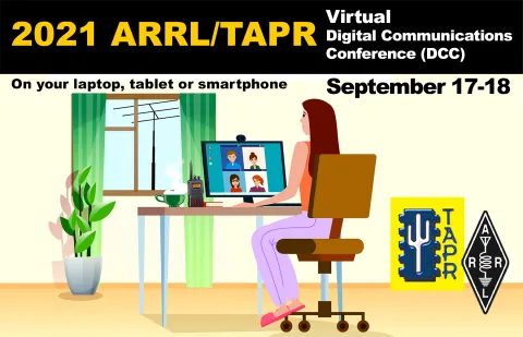
The 40th annual ARRL and TAPR Digital Communications Conference (DCC) will take place September 17–18, 2021. Due to the coronavirus pandemic, this year’s conference will be held online. Registered DCC attendees participating via Zoom will be able to interact with presenters and other attendees via a chat room as well as raise a virtual hand to ask questions. Click here to register (you don’t need a Zoom account to register). Non-registered DCC attendees can watch the live stream for free on YouTube and can chat and ask questions via the moderator monitoring the channel. No registration is required for YouTube access (the YouTube URL will be announced and posted on this webpage preceding the DCC). DCC registration is free for TAPR members and $30 for non-members. Members receive a 100% discount at checkout. Click here to register. Non-members who would like to join TAPR and receive the free DCC pass can simply add TAPR membership and DCC registration to their shopping carts. After checkout, they will receive the free DCC pass when their membership is processed.
Call for Papers and Speakers: Technical papers are being solicited for presentation. Papers will also be published in the Conference Proceedings. Authors do not need to participate in the conference to have their papers included in the Proceedings. The submission deadline is August 15, 2020. Submit papers via email to Maty Weinberg, KB1EIB, [email protected]. Papers will be published exactly as submitted, and authors will retain all rights.
Conference papers will be distributed as pdf’s to participants. Printed copies of the papers will be available for sale at Lulu (http TBD).
Also, speakers are invited to make presentations on topics of interest without submitting papers for the Conference Proceedings.
All speakers and presenters must contact Steve Bible, N7HPR <n7hpr @ tapr.org> to reserve a slot for a presentation. Indicate whether you need a 15- or 30-minute slot and if you need to present on a specific day (Friday, September 17 or Saturday, September 18). A pre-recorded presentation can be submitted in lieu of a live virtual presentation.
Paper and presentation topic areas include, but are not limited to software defined radio (SDR), digital voice, digital satellite communication, digital signal processing (DSP), HF digital modes, adapting IEEE 802.11 systems for Amateur Radio, Global Positioning System (GPS), Automatic Position Reporting System (APRS), Linux in Amateur Radio, AX.25 updates, Internet operability with Amateur Radio networks, TCP/IP networking over Amateur Radio, mesh and peer-to-peer wireless networking, emergency and homeland defense backup digital communications in Amateur Radio.
Lightning Talks
Ad hoc “lightning talks” on various topics of interest will be announced throughout the DCC. Registered attendees will be able to participate in any lightning talk that whets their appetite.
Hardware and Software Demos
Hardware and software demonstrations will be conducted during the DCC by means of Zoom’s breakout room feature.
The magnetic sensor for the PSWS project is an off-the-shelf, low-cost ($20) magnetic sensor using a new technology (“magneto-inductive”) with a noise floor of 4 pT/sqrt(Hz) at 1 Hz (PNI Geomagnetic Sensor RM3100, visit the website for more details). Regoli et al. (2018) demonstrated that the sensor performance is adequate for both space-borne and ground-based applications to study geomagnetic activity. Given that the sensor will be located in various electromagnetic environments, we expect the performance to be somewhat compromised and thus our target level is ~10 nT.
The RM3100 MI magnetometer consists of 1) single board computer (i.e. Raspberry Pi 3); 2) local magnetometer support board extender; and 3) remote magnetometer support board extender (see Figure 1). The remote board (Item #3) contains the RM3100 sensor which needs to be placed outside away from any sources of EMI while both the computer and local board are located inside. A recommended cable between the local and remote boards is a CAT5E or CAT6A shielded twisted pair (solid copper, NOT high resistance copper coated aluminum (CCA)).
The magnetometer package is expected to be in the range of $100 to $150. Again, the performance level of the magnetometer is lower (field resolution, in particular) than that of the high-performance, science-grade magnetometers deployed at geophysical observatories across the US. We note, however, that the proposed network is focused primarily on their spacing to increase the spatial resolution. Given the adequate resolution level (< 10 nT at 1 Hz), most of the major geomagnetic activity (e.g., geomagnetic storms, substorms (may be limited to high-latitude regions) and large-scale ULF waves/disturbances) is expected to be observed, which will be compared with the HF measurements.
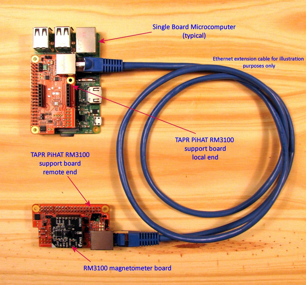
Figure 1. A RM3100 MI magnetometer system (TAPR PiHAT version).
Magnetic Sensor Packaging
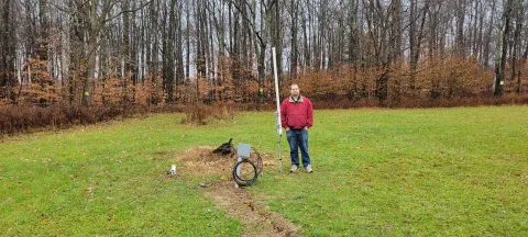
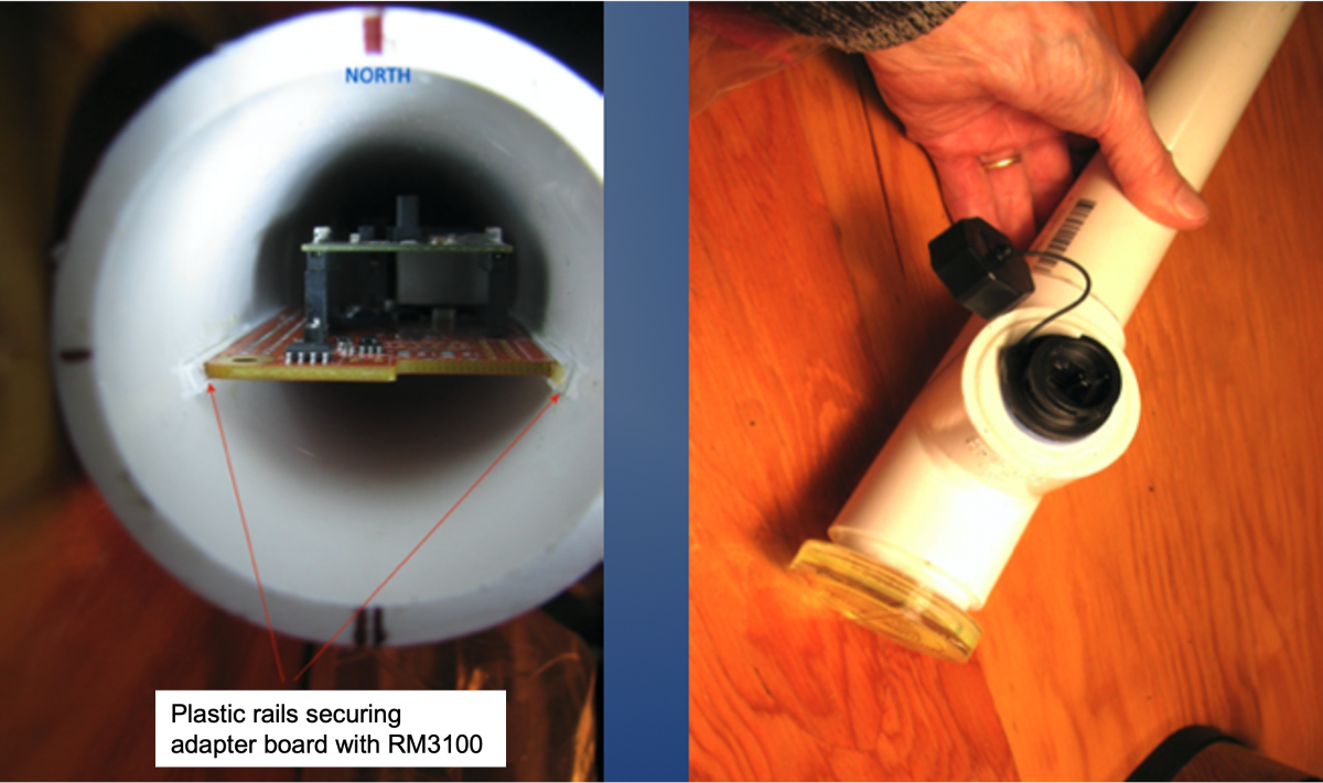
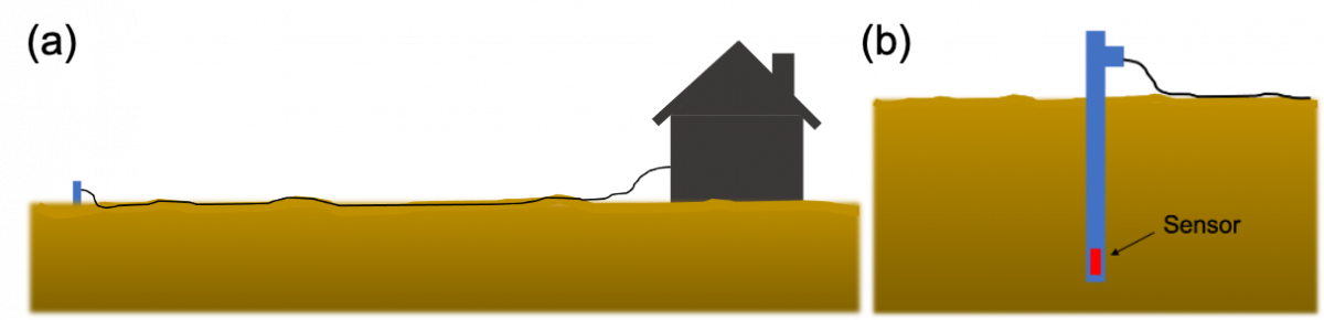
The sensor board (Item #3: remote magnetometer support board extender) is housed in a PVC pipe structure as shown in Figure 2 for weather protection. It can be positioned vertically under the ground so that the sensor, located on the bottom of the pipe, is well below the ground surface level, providing stable temperature (Figure 3). Field installation is shown in Figure 4. Its construction is detailed in a separate document (RM3100 magnetometer assembly in PVC pipe-1.pdf).
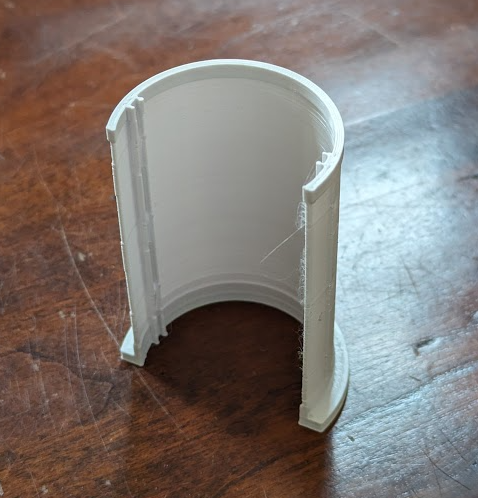
Note1 (April, 2026): A 3D-printed solution for mounting the sensor board in a 2 inch SCH40 plastic pipe now exists. See images here and the STL file for 3D printing here (right click to download). (Thanks to Majid Mokhtari, University of Scranton, for this design.)
Note 2 (April, 2026): A 3D-printed solution for mounting the sensor board in a 1.5 inch SCH40 plastic pipe now exists. See image here. The SCAD file is here and the STL file for 3D printing here (right click to download). (Thanks to Philip Gladstone, N1DQ, for this design.)
Installation and Alignment
The PVC sensor housing is installed outside of the building where the host computer is located (Figure 3(a)). It is recommended that the sensor is placed at a sufficient distance to avoid any possible EMI source (e.g., the building). A minimum recommended cable length is 100 ft. In an area where EM noise is a concern, use a longer cable (depending on the nature of the noise source). CAT5E and CAT6A can support up to 400 ft and 500 ft, respectively. The cable should be rated for direct burial. The PVC sensor housing is positioned vertically, leaving only the upper part of it (approximately 10 inches) above the ground surface as shown in Figure 3(b) and Figure 4. This provides temperature stability.
The sensor should be oriented in compliance with the widely accepted geomagnetic coordinate system, “HEZ”, in which H points toward the local geomagnetic north in the horizontal plane (perpendicular to the line pointing toward the center of the earth defined as Z). E completes the orthogonal system, pointing toward the geomagnetic east. Thus, Z = H x E in a vector form. Simply, H is defined as a direction which a compass needle would point toward. Figure 4 shows the definition of the coordinate system and the sensor installation conforming to this. It should be noted that the sensor's original XYZ coordinates do not match the HEZ coordinates because of how it is oriented in the pipe (the sensor was designed for use in the horizontal plane, but we are installing it in the vertical plane). Thus, a reallocation of coordinates is required in the post-processing data processing algorithm. That is, H = -Z, E = Y and Z = X where X, Y and Z are the original tri-axial components of the sensor output while H, E and Z are the local geomagnetic components that will be used for scientific use.
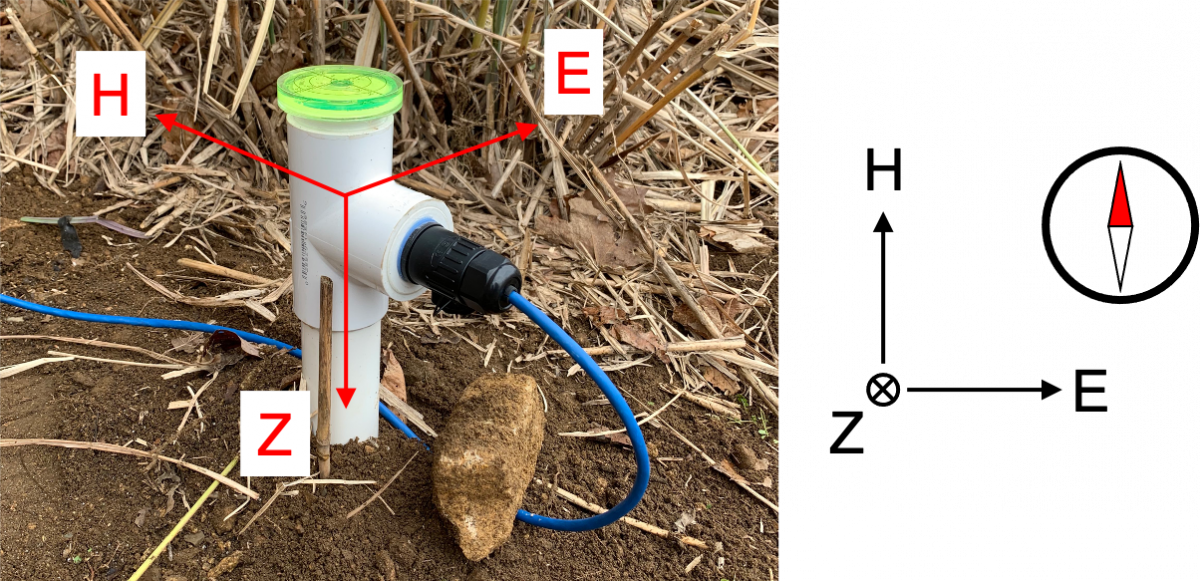
Figure 4. RM3100 sensor PVC pipe packaging installed on the ground.
Initial Data Verification
A “quick and dirty” way to ensure the operation and data quality of the installed magnetometer is to compare the data with the predicted values from a model called International Geomagnetic Reference Field (IGRF), an approximate model field at a particular location. The IGRF can be obtained on a user-friendly website run by Kyoto University. The only information necessary for the model field is the geographic coordinates and altitudes of the magnetometer location and the year of interest. Figure 5 presents a snapshot of the website for model magnetic field at Hope, New Jersey (41N, 75W). The altitude does not need to be very accurate (0 m was entered in this case). It is important to note that the “northward (X)” and “eastward (Y)” in the IGRF are different from our “H” and “E” as the IGRF reports “geographic” north and east whereas our system reports “geomagnetic” north and east. Thus these two values should NOT be compared directly. They are related by X = H * cos (D) where D is declination, the angle on the horizontal plane between magnetic north and true north. Nevertheless, the total “horizontal” field should be close to each other: that is, horizontal = sqrt(X2+Y2) = sqrt(H2+E2). Likewise, the “downward (Z)” should also be close. In addition, the total field can be compared to see if they are similar, as defined as sqrt(X2+Y2+Z2) = sqrt(H2+E2+Z2). Note this is labeled as “F” (total intensity) on the IGRF website. The IGRF values are only from a model and thus it is natural that there are some discrepancies between the actual measurements and the IGRF values. This can be more extreme at high latitudes and/or during geomagnetically disturbed times.
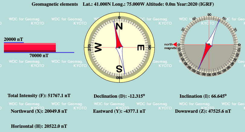
Figure 5. An example of IGRF model magnetic field at Hope, New Jersey (41N, 75W, 0-m altitude) in 2020.
Regoli, L. H., Moldwin, M. B., Pellioni, M., Bronner, B., Hite, K., Sheinker, A., and Ponder, B. M.: Investigation of a low-cost magneto-inductive magnetometer for space science applications, Geosci. Instrum. Method. Data Syst., 7, 129–142, https://doi.org/10.5194/gi-7-129-2018, 2018.
The HamSCI Magnetometer Documentation is © Author(s) 2023. This work is distributed under the Creative Commons Attribution 4.0 License.
For more information about scientific modulation on WWV, email [email protected].
HamSCI's WWV/H Scientific Modulation Working Group is exploring possibilities for additions to WWV and WWVH's modulation that can be used for science purposes. For updates on this project, join the Google Group here: https://groups.google.com/g/wwv-h_scie
Thanks KE0KA for this fantastic presentation of our characterization signal:
A characterization signal has been designed for test broadcasts on WWV and WWVH. View it here: 
Aidan KB3UMD has ported the signal generation code to Python (note that the pseudorandom sequences are not the same): https://github.com/aidanmontare-edu/wwv-h-characterization-signal-ports
______________________________________________________________________________________________________________________________________________________________________________
TAPR DCC Presentation, 18 September 2021:
WW0WWV has written an excellent report on the TAPR presentation, which you can read here: WWV/WWVH Scientific Modulation Working Group | WWVARC
1 November 2021: An announcement about the characterization signal has been added to WWV and WWVH! The signal is scheduled to begin at Minute 8 on WWV and Minute 48 on WWVH, starting on November 15.
Looking for campaign information? See www.hamsci.org/sunrisefest.
If you would like to make recordings using your SDR: We recommend making I/Q recordings, centered on a WWV frequency (2.5, 5, 10, 15, 20 MHz), with a sampling rate above 20 kS/sec.
If you have a KiwiSDR that you are willing to let us use for remote recording, please email [email protected].
You can upload files and notes here:
Interested in analyzing our characterization signal? Here are some KiwiSDR recordings from Fort Collins, made using N6GN's KiwiSDR: 
Besides auroral observations, magnetic field measurements are one of the traditional ways of observing the space weather phenomena on the ground. To that end, magnetic sensors, “magnetometer”, are typically used for space research. The instrument has a wide range of applications including metal detection, non-contact switch, non-destructive testing, oil/coal exploration, military as well as space research. Among many types of magnetometers, induction magnetometers (“fluxgate” and “search-coil”) are widely used for space applications because their designs are relatively simple and yet reliable, providing excellent performance level. For the HAMSci space weather station project, proposed is an inexpensive, simple, mid-grade magnetometer utilizing the anisotropic magneto-resistive (AMR), magneto-inductive and fluxgate technologies.
The magnetic fields at the Earth’s surface range from 25,000 nT to 65,000 nT. Observations of absolute magnetic field values are critical in geological studies. In space research, however, only variations are of major interest. The range varies depending on the strength of the activities, from hundreds of nano-Tesla (nT) to as small as a fraction of nT. A proposed magnetometer should be able to measure the earth’s magnetic field variations associated with various geospace activities. Thus, measurements of the background magnetic fields can be ignored (oftentimes, the background fields are removed or subtracted). Figure 1 presents an example of magnetic field data from ground-based stations (top panel: Ottawa, ON; bottom panel: Fredericksburg, VA). Note that the background magnetic fields were removed in these data sets. One of the important parameters is resolution. Many science-grade magnetometers provide a fraction of nT resolution near DC. Very high-end ones can go as small as tens of pT resolution or lower. For the HAMSci space weather station project, a mid-range performance level will be targeted, adequate to measure large- and medium-scale geomagnetic activities approximately from a few to hundreds of nT. Although sub-nT measurements may be technologically achievable for this project, much more sophisticated construction, calibration and installation are required. Some of the important hardware requirements for the project are shown as follows:
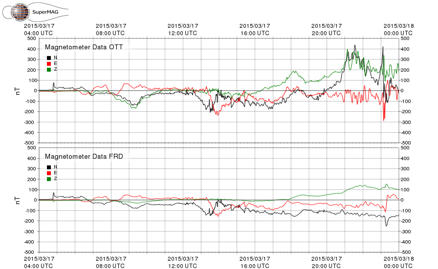
Figure 1. Example data from ground magnetometers (top: Ottawa, ON; bottom: Fredericksburg, VA).
|
Type |
Pros |
Cons |
Example Product |
|
Magneto-Resistive (MR) |
|
|
|
|
Anisotropic Magneto-Resistive (AMR) |
|
|
|
|
Magneto-Inductive (MI) |
|
|
|
|
Fluxgate |
|
|
|
Sensors can be built from scratch by hand (in accord very much with the “HAMScism”). The sensor consists of magnetic core material and magnet wire around it. Most of electronic components are inexpensive (can be either analog or digital). Although material/part costs are low, the project can be labor-intensive (coil winding, machining, electronics fabrication, test/calibration). Quality control can be challenging because sensors need to be accurately calibrated)
A proper installation/operation guideline is necessary to guarantee good quality data. Sensors need to be located in an electromagnetically-clean environment. For this, a passive method is typically used by placing the sensor away from any EMI sources using a cable (typically tens of meters from the station building). If there is a powerful radio transmitter around it, an aggressive low-pass filter may be necessary. A careful sensor orientation is required. Stable temperature is also highly desired (for fluxgate types, whether MR/AMR sensors are temperature-sensitive needs to be investigated). For details, go to Installation and Operation Page.
Радиосигналы отражаются от изменчивой ионосферы. Различные сигналы радиостанции национального бюро стандартов в Вашингтоне WWV, отражаясь от ионосферы, претерпевают изменения в длине волны и в концентрации электронов. Это приводит к изменениям в наблюдаемой частоте радиосигналов, сродни нарастанию и падению высоты тона свистка проезжающего поезда.
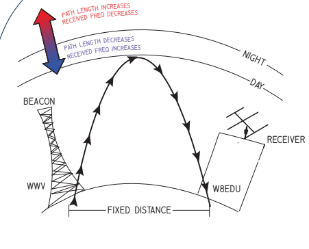
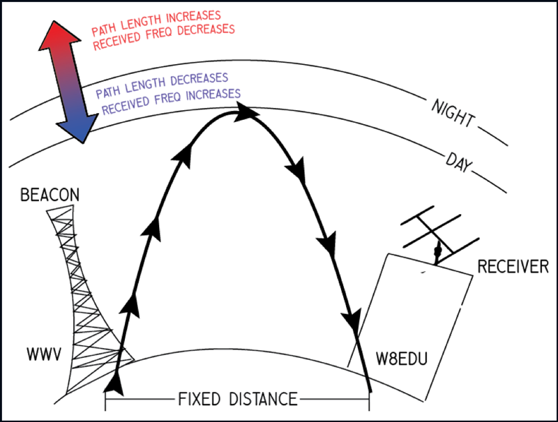
На данном рисунке изображён процесс того, как сигналы радиостанции Бюро Стандартов США отражаются от ионосферы. Космическая погода влияет на то, как далеко распространяется сигнал, прежде чем он изменит направление, и принимающая станция определяет это как изменение частоты сигнала.
Сравнение принятого радиосигнала с точным местным стандартом частоты, таким как осциллятор, управляемый GPS, позволяет пользователю измерить эти ионосферные сдвиги частоты. Это измерение подготовлено и записано с помощью программного обеспечения с открытым исходным кодом. Многочисленные наборы данных, записанные одновременно из нескольких мест, предлагают информацию - когда эти наборы данных исследуются как по отдельности, так и вместе - об ионосфере во время сбора данных. Эта информация включает перемещение ионосферных возмущений и другие важные явления в различных масштабах.
Вы можете узнать больше о том, как работают эти измерения, пройдя по ссылке.
Сбор доплеровских данных с вашей станции
Есть два способа собрать доплеровские данные из местоположения вашей радиостанции. Один из них - это сбор данных .CSV с помощью программы частотного анализа - данный метод наиболее подходит для для долгосрочного сбора данных. Другой - сбор аудиофайлов, что рекомендуется только для краткосрочных экспериментов, таких как фестивали затмений (eclipse festivals).
Вам понадобится:
КВ-радио и антенна, способная принимать сигналы от станций стандартного времени (частоты и времени)
Компьютер
Звуковой адаптер, подобный этому, для подключения компьютера к радио. (Как проверить что ваш звуковой адаптер подходит к радио?)
Осцилляттор с функцией GPS (здесь и далее - GPSDO), подобный этому, для обеспечения точности ваших измерений.
Способ подключения GPSDO к вашему радио будет зависеть от того, какой у вас тип радио.
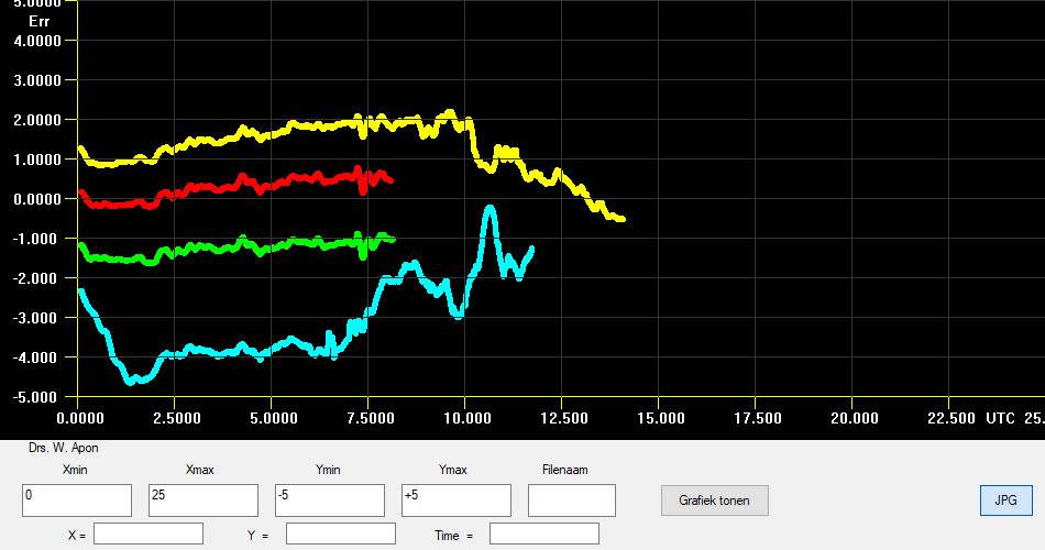
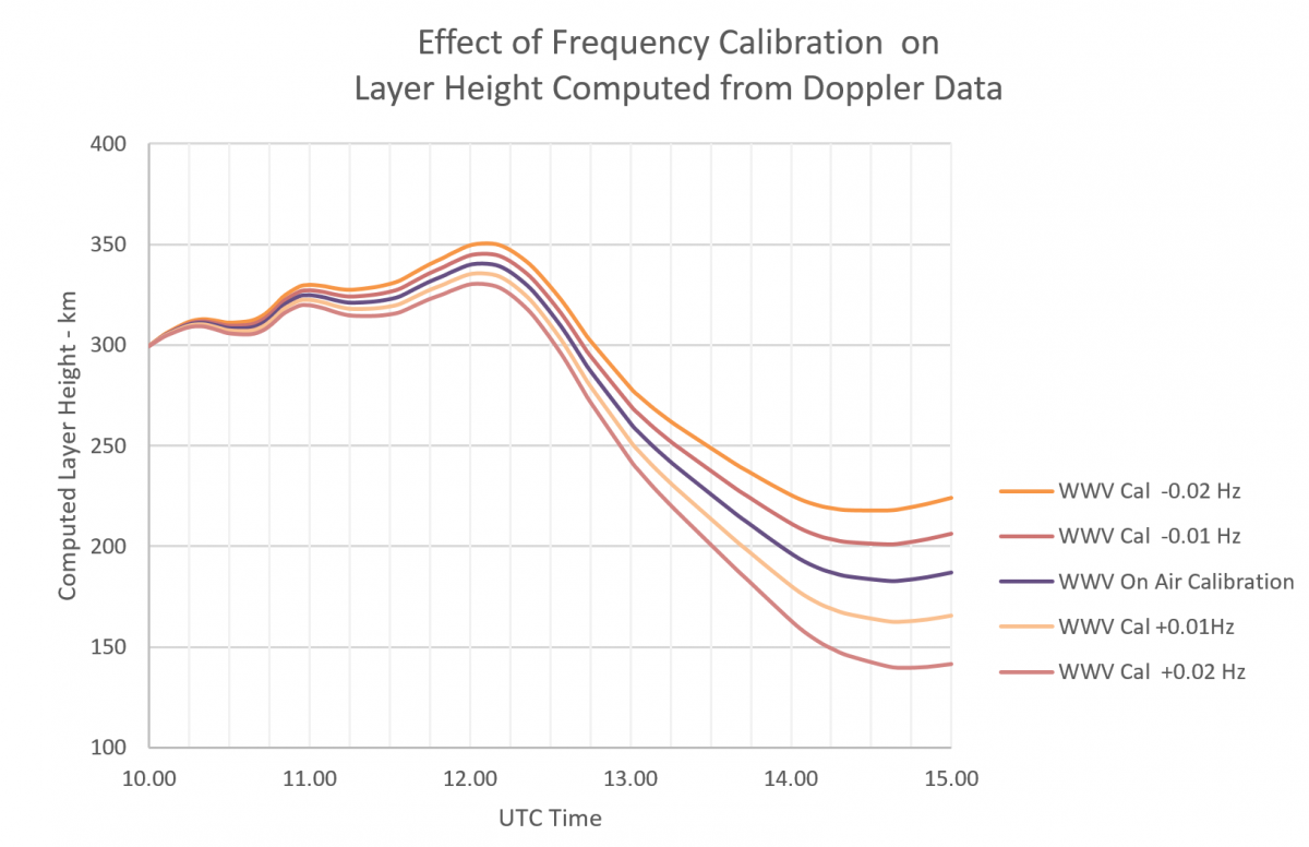
Можно собирать данные без GPSDO, но с ним ваши измерения будут намного лучше. Хотя вы сможете увидеть тенденции в своих данных, вы не сможете сделать количественную оценку высоты слоя. Как показывает эта диаграмма Стива Сервина WA5FRF, небольшая ошибка в частоте вашего осциллятора приводит к большой ошибке со временем при оценке высоты слоя:
Выбор частоты радиомаяка
Вам будет нужна частота радиомаяка, которую можно услышать с вашей станции. В примерах на этой странице используется частота 10 МГц. Вы можете найти список радиостанций стандартного времени здесь.
Мировые радиостанции, передающие сигналы точного времени на короткой волне, которые можно использовать для Фестиваля измерения частоты затмений:
|
Африка |
Отсутствуют радиостанции КВ диапазона.
|
|
Азия |
* Радиопозывной BPM, Китай, Шэньси, Пучэн (Центральный Китай) 2,50 МГц, 5,0 МГц, 10 МГц, 15 МГц (мощность в кВт неизвестна для каждой частоты) * Радиопозывной HLA, Южная Корея, Тэджон 5,0 МГц (2 кВт) |
|
Европа |
* Радиопозывной RWM, Россия, Москва, Талдом (Восток Европы) 4,996 МГц (10 кВт), 9,996 МГц (10 кВт), 14,996 МГц (10 кВт) |
|
Северная Америка |
* Радиопозывной WWV, США, Колорадо, недалеко от Форт-Коллинза (центральные Соединенные Штаты Америки) 2,50 МГц (2,5 кВт), 5,0 МГц (10 кВт), 10,0 МГц (10 кВт), 15,0 МГц (10 кВт), 20 МГц (2,5 кВт), 25 МГц (2,5 кВт) * Радиопозывной CHU, Канада, Онтарио, Оттава (на юго-востоке Канады) 3,33 МГц (3 кВт), 7,85 МГц (10 кВт), 14,67 МГц (3 кВт) |
|
Океания |
Нет коротковолновых радиостанций. Используйте WWVH на Гавайях или BPM в Китае |
|
Тихий океан |
* Радиопозывной WWVH, США, Гавайи, Кекаха (в центре северной части Тихого океана) 2,50 МГц (5 кВт), 5,0 МГц (10 кВт), 10,0 МГц (10 кВт), 15,0 МГц (10 кВт) |
|
Южная Америка |
* Радиопозывной LOL, Аргентина, Буэнос-Айрес 10 МГц (2 кВт) * Радиопозывной PPE, Бразилия, Рио-де-Жанейро, Рио-де-Жанейро 10,0 МГц (1 кВт) * Радиопозывной YVTO, Венесуэла, Каракас 5,0 МГц (1 кВт) |
Рекомендации по выбору лучшей радиостанции:
1) используйте ближайший радиомаяк на вашем континенте
2) если можете, используйте частоту с наибольшей мощностью (в кВт)
3) рекомендации для выбора частоты приема:
Для континентальной и национальной радиосвязи попробуйте
- ночью: полоса частот 3 МГц - 9 МГц,
- днем: полоса частот 5 МГц - 16 МГц.
По региональной и ведомственной радиосвязи попробуйте
- ночью: полоса част 0,3 МГц - 5 МГц в Европе, полоса частот 2 МГц - 6 МГц в тропиках,
- днем: полоса частот 0,3 МГц - 8 МГц в Европе, полоса частот 4 МГц - 12 МГц в тропиках.
Более подробная информация по частотным диапазонам:
Распространение электромагнитных волн зависит, конечно, от среды, но также и от частоты. Приведенные ниже диапазоны даны для справки, условия распространения в ионосфере сильно различаются в зависимости от солнечного цикла, времени года, региона мира, времени суток, схем радиоприёмных устройств ...
Ниже 4 МГц: связь обычно возможна только на большом расстоянии в темноте между местом передачи и приема, после исчезновения слоя D. Земная волна выполняет преобладающую функцию, особенно на частотах ниже 1 МГц. Отличная региональная полоса в начале и в конце дня с дальностью до 600 км (до 2000 км в зависимости от условий). Местное сообщение может осуществляться в радиусе нескольких десятков километров. Связь возможна без длины скачка в излучении NVIS.
От 4 до 8 МГц: возможна межконтинентальная связь (более 4000 км), но стабильная связь обычно возможна от 200 до 3000 км. Местное сообщение возможно на расстоянии до тридцати километров. Возможна связь без «мертвой зоны» в излучении NVIS (пространственная волна с квази-вертикальным падением) с дальностью менее 400 км для самых низких частот этой части спектра.
8–12 МГц: круглосуточный доступ для континентальной связи. Длина скачка радиосигнала от 300 км днем до 1000 км ночью. Межконтинентальная связь возможна в темное время суток между местом излучения и приема.
От 12 до 16 МГц: диапазон открыт в течение дня с дальностью до 2000 км в любое время. Связь возможна с антиподами в благоприятные периоды солнечного цикла. Длина скачка радиосигнала от 200 км днем до 1600 км ночью.
Мы просим вас использовать пакет программного обеспечения с открытым исходным кодом fldigi версии не старше 4.1.13. В режиме «частотного анализа» ежедневно создаются файлы отклонений частоты, автоматически называемые «analysis_(date).csv». Он будет в каталоге /fldigi/ temp /, или .fldigi / temp /, или в каком-либо эквиваленте. Вы должны использовать последнюю версию fldigi, иначе ваши данные будут перезаписаны.
Скачайте fldigi, установите, убедитесь, что он работает правильно. Найдите модуль «Частотный анализ» (англ. Freq Analysis) в раскрывающемся меню «Рабочий режим» (Op Mode).
Настройте свое радио (в режиме AM) на станцию стандарта времени на 10 МГц и определите, какую из них вы можете легко измерить.
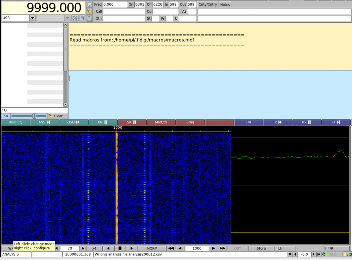
Выберите режим с использованием верхней боковой полосы вашего приемника (USB) и настройтесь на частоту на 1 кГц ниже несущей. Для 10 МГц настройтесь на 9,999 МГц (9999,000 кГц - см. Изображение) и слушайте тон 1000 Гц.
В fldigi убедитесь, что настроенная частота в верхнем левом углу совпадает с частотой вашего радио. Чтобы изменить его, щелкните верхнюю половину цифры, чтобы увеличить, или нижнюю половину, чтобы уменьшить.
Ищите линию 1000 Гц на водопадной диаграмме Флдиги. Щелкните там курсором или используйте поле настройки частоты в нижней части экрана fldigi. Вы должны установить значение в поле в нижней части экрана ровно 1000. (Если fldigi не принимает этот ввод должным образом, попробуйте начать запись, а затем установите значение 1000).
В fldigi выберите меню «Op Mode» и выберите режим «Freq Analysis».
Найдите «запись CSV-файла» в нижней строке fldigi слева. Если у вас чистый сигнал и вы видите только одну несущую, вы должны увидеть красивый график в конце дня. Если вы видите несколько несущих, может потребоваться более подробная информация о доплеровском режиме.
Теперь оставьте fldigi в покое. Во время сбора данных оставьте радио в покое и убедитесь, что компьютер не выключен из-за автоматического обновления.
По окончании периода записи закройте файл fldigi. Файл «analysis.csv» должен находиться в вашем каталоге / fldigi / temp /. В качестве альтернативы они могут находиться в "/fldigi.files/analysis". В MacOS они находятся в скрытом каталоге ~ / .fldigi / analysis - чтобы найти их, вы должны отобразить файлы с помощью CMD + SHIFT +. в Finder. В конце периода сбора данных у вас должен быть один файл “analysis- * .csv” на каждый день записи данных. Пожалуйста, переименуйте эти файлы, добавив свое имя или позывной: например, analysis_200620 - W8EDU.csv. Не редактируйте содержимое файлов.
Примечание: Этот подход предназначен для краткосрочного сбора данных, например, во время фестивалей затмений (eclipse festivals). Для долгосрочного сбора данных мы рекомендуем использовать способ, описанный выше.
1) Подключите радиоприёмник к звуковой карте компьютера.
Если вы управляете своим радио через fldigi или flrig, вы уже знаете, как это сделать. Инструкции могут различаться в зависимости от типа радиоприёмника. Если вам нужна внешняя звуковая карта USB, мы рекомендуем эту: https: //www.amazon.com/gp/product/B00IRVQ0F8/ref=ppx_yo_dt_b_asin_title _...
2) Скачайте программу Audacity.
Audacity - это хорошо зарекомендовавшая себя программа с открытым исходным кодом для записи звуков. Вы можете скачать её здесь: https://www.audacityteam.org/download/
Программу можно установить сразу на русском языке. Можно также поменять язык, выбрав вкладку «Правка»> «Настройки»> «Interface». Если установлен интерфейс на английском языке, чтобы поменять язык, необходимо выбрать вкладку Edit>Preferences>Interface ().
3) Настройте метаданные Audacity.
Загрузите этот XML-шаблон и запишите каталог, в который он загружается: EclipseTags.xml
В разделе «Правка»> «Метаданные» нажмите «Загрузить» и выберите файл, затем отредактируйте его, чтобы он соответствовал вашей радиостанции .. (Вы также можете добавить метаданные вручную, используя список ниже.)
[рисунок]
В Audacity перейдите к вкладке «Правка»> «Метаданные» (Edit> Metadata) и заполните следующие поля:
В поле «Исполнитель» введите свой позывной. (Если вы слушатель коротких волн, а не радиолюбитель, используйте свое имя или позывной SWL.)
В поле «Название альбома» введите название события, например «Затмение в декабре 2020 года».
В поле «Год», укажите текущий год.
В поле «Жанр» укажите модель вашего радио.
Добавьте вручную и заполните следующие поля.
Адрес электронной почты
Любительская радиостанция
Антенна
Звуковая карта
Частота
Автоматическая Регулировка Усиления AGC (Automatic Gain Control) (вкл. или выкл.)
Широта (используйте десятичные дроби, а не минуты и секунды!)
Долгота
Высота над уровнем моря (м)
Часовой пояс (пример формата: UTC-05: 00)
Квадрат сетки координат
Страна
ВАЖНО: Если у вас есть несколько радиостанций, собирающих данные одновременно под одним позывным, добавьте дефис и номер станции для каждой станции, в тех случаях когда вы бы использовали позывной. Например, если станция W8EDU одновременно выполняет сбор данных на радиостанции Flex и радиостанции Icom, пометьте одну как W8EDU-1, а другую как W8EDU-2, добавьте комментарий в метаданные для каждой станции, объясняющий, что оператор запустил несколько станций и убедитесь, что метаданные верны и полны. Это упростит сортировку данных эксперимента на этапе анализа.
Нажмите «Сохранить» и сохраните файл XML, затем нажмите «Установить по умолчанию».
Установите флажок «Не показывать при экспорте аудио», затем нажмите «ОК».
4) Установите настройки записи.
Откройте вкладку «Запись» в меню «Настройки» («Правка»> «Настройки»> «Запись»). Снимите флажок «Проигрывать другие треки во время записи (наложение)» и установите флажки «Записывать новый трек» и «Обнаруживать потери сигнала».
В поле «Имя для вновь записанных треков» введите свой позывной, затем один знак подчеркивания, а затем букву, соответствующую вашему часовому поясу в этом списке: [https://en.wikipedia.org/wiki/List_of_military_time_zones]
Например, станция W8EDU находится в восточном стандартном времени (UTC - 05:00), что соответствует букве R, поэтому правильное название трека будет начинаться с «W8EDU_R_». (Если вы находитесь в неполном часовом поясе, используйте букву J; чтобы отметить, что ваши данные нуждаются в ручной обработке в зависимости от вашего местоположения.)
Добавьте частоту местного осциллятора вашего радио. Например, если W8EDU настроен на 9,999 МГц для прослушивания радиостанции Бюро стандартов США WWV на частоте 10 МГц, в поле «Заданное имя трека» должно быть указано «W8EDU_R_9999kHz_». Если W8EDU настроен на 9,995 МГц для наблюдения за радиостанции RWM на частоте 9,996 МГц, в поле «Заданное имя трека» должно быть указано «W8EDU_R_9995kHz_». Эта инструкция была добавлена для фестиваля затмений в июне 2021 года и поэтому её нет на скриншотах ниже.
Убедитесь, что установлены флажки в полях «Системная дата» и «Системное время». Когда вы закончите, окно должно выглядеть так:
В разделе «Качество» > «Формат сэмплов по умолчанию» установите значение 16-бит. В поле «Частота дискретизации по умолчанию» (Default Sample Rate) установите значение 8000 Гц (если вашему приемнику не требуется более высокая частота, как описано в Шаге 2 выше).
Откройте вкладку «Устройства» в меню настроек и убедитесь, что вы записываете со своего радио, а не с микрофона вашего компьютера или другого источника.
Когда закончите, нажмите ОК.
5) Установите настройки записи и сделайте тестовую запись.
В середине верхней панели инструментов, в ниспадающем меню, выберите значение «1 канал записи (моно)».
Убедитесь, что частота вашего проекта установлена на 8000 Гц в ниспадающем меню в нижнем левом углу экрана.
Настройте аудиовход на звуковую карту, подключенную к вашему радио. Имена устройств могут отличаться. Возможно, вам придется поэкспериментировать, чтобы убедиться, что источник, с которого вы записываете, правильный.
Нажмите кнопку записи ⬤; вы должны увидеть начало записи первого трека с правильным названием трека и отметкой времени. Если название трека неправильное, попробуйте перезагрузить компьютер и начать запись снова.
Нажмите кнопку стоп ⏹️, затем снова запишите ⬤. На этот раз вы должны увидеть второй трек. Название на каждом треке будет соответствовать началу времени его записи.
(рисунок)
Обратите внимание на «Оставшееся дисковое пространство для записи» внизу экрана. Одна неделя записи составляет 168 часов, поэтому вам может потребоваться приостановить и перезапустить сбор данных во время эксперимента. Оценка также может быть не совсем точной. Ознакомьтесь с документацией Audacity по длине записи здесь.
6) Сохраните проект.
Обязательно остановите запись ⏹️, прежде чем продолжить.
Сохраните проект (Файл> Сохранить проект). Это позволит компьютеру сохранить ваши настройки. Вы можете увидеть окно с вопросом, хотите ли вы сохранить проект, даже если в нем нет треков: нажмите OK.
7) Убедитесь, что ваши файлы WAV сохраняются правильно.
Создайте каталог для сохранения файлов в соответствии со следующим правилом «<Callsign> _Eclipse_Dec2020». Например: W8EDU_Eclipse_Dec2020. (Если вы запускаете одновременный сбор данных на нескольких радиостанциях, используйте идентификатор с переносом, описанный в пункте 3.)
Перейдите в Файл> Экспорт> В несколько файлов. Выберите каталог, в который вы хотите сохранить файлы. В разделе «Имена файлов» убедитесь, что выбран вариант «Используется метка / имя трека».
Нажмите кнопку «Экспорт». Откроется диалоговое окно, подтверждающее, что каждый трек был сохранен в отдельный файл в формате WAV. (Примечание: если ваши файлы слишком велики для экспорта, см. раздел «Часто задаваемые вопросы» ниже.)
Когда это будет сделано, вы можете удалить свои тестовые треки, щелкнув кнопку X в верхнем левом углу трека.
Когда вы откроете каталог, вы должны увидеть метаданные исполнителя и альбома. Убедитесь, что имена ваших файлов имеют правильный формат: например, «W8EDU_R_9.999MHz_2020-10-23_22-36-18.wav».
Вы должны записывать свои данные на диск, на котором есть не менее 10 ГБ свободной области памяти. Если вы работаете в Windows, перейдите в каталог данных и активируйте сжатие: Свойства -> Общие -> Дополнительно -> Сжать содержимое для экономии места на диске. (См. снимок экрана ниже).
8) Дополнительно: откалибровать аудиовыход для записи файла .WAV
Мы заинтересованы в сборе данных об амплитуде, где это возможно; Вы можете прочитать больше об этом здесь. Если в вашем радио есть цепь Автоматической Регулировки Усиления (АРУ), которую можно отключить, и отдельную регулировку усиления высоких частот, вы также можете собирать данные об амплитуде. Однако недостаточно просто выключить AGC; вы должны установить усиление высоких частот на соответствующий уровень. В противном случае уровень звука будет почти постоянным независимо от силы сигнала, и данные могут быть скомпрометированы. После выключения АРУ необходимо установить регулятор усиления высоких частот приемника таким образом, чтобы уровень звука давал измеримые амплитуды, которые никогда не выходят на полную шкалу, не зажимаются или ограничиваются. Для этого необходимо предварительное тестирование, чтобы убедиться, что максимальная мощность сигнала не приводит к перегрузке входа звуковой карты. Если ваше радио не соответствует этим требованиям, перейдите к пункту 9 ниже.
Вот способ настройки приемника:
При включенной АРУ настройте радиомодуль на воспроизведение тона 1000 Гц в режиме USB, настроив радиомодуль на 1 кГц ниже несущей частоты (например, 9,999 МГц для несущей частоты 10 МГц).
Установите регулятор громкости приемника на комфортный уровень прослушивания, используя обычный динамик радио или наушники. Он должен быть достаточно громким, чтобы быть выше шума приемника при отсутствии сигнала, но не настолько громким, чтобы вызывать искажения.
Установите уровень записи в Audacity, чтобы получить примерно 1 / 4-1 / 2 уровня записи полной шкалы, или на уровне, который оставляет от 6 дБ до 10 дБ запас по уровню ниже полной шкалы.
Выключите АРУ приемника.
Используйте регулятор усиления высоких частот, чтобы установить выходной аудиосигнал на тот же уровень, что и при включенной АРУ.
Сделайте дневную запись и изучите ее. Если уровни достигли полной шкалы в любой момент во время записи, уменьшите регулировку усиления высоких частот и попробуйте еще раз. Идея заключается в том, чтобы иметь достаточное усиление радиочастоты, чтобы получить измеримые уровни сигнала даже в самое слабое время дня, но не настолько, чтобы амплитуда в наиболее сильном периоде дня достигла максимума или плоских вершин на полной шкале.
После того, как усиление высоких частот установлено, его нельзя изменять во время записи данных о затмении.
При отправке вашей анкеты ниже, не забудьте указать, что вы выполнили эту процедуру.
9) Все готово!
Теперь у вас все готово для сбора данных! Если вам нужно возобновить сбор данных в любое время, нажмите кнопку остановки записи и следуйте пункту 7 выше.
Когда все будет готово, ваша установка должна выглядеть примерно так:
Анализируйте ваши данные
Вы можете построить график данных с течением времени, чтобы увидеть геофизические изменения. Если вы получите четкий сигнал, восход солнца должен четко отображаться в ваших частотных данных.
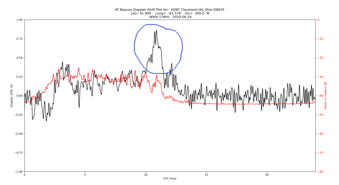
При помощи графика вы сможете отслеживать ежедневные изменения. Если вы построите график данных за длительный период, вы увидите утренний пиковый сдвиг с изменяющейся продолжительностью дня.
Хороший способ проверить достоверность ваших данных: попросите знакомых или друзей поблизости, чтобы они снимали данные на тех же частотах. Это поможет отделить локальный шум в вашей среде от сигналов геофизического характера. На графике ниже все станции находятся в пределах 5 км друг от друга, и все три станции наверху имеют осцилляторы с функцией GPS. (Изображение предоставлено: Wim PA0SLT)
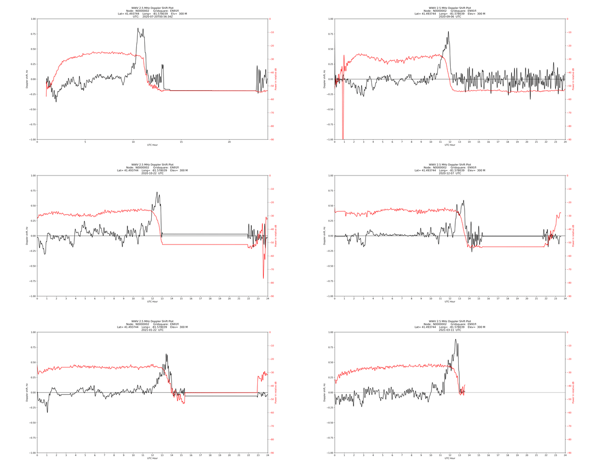
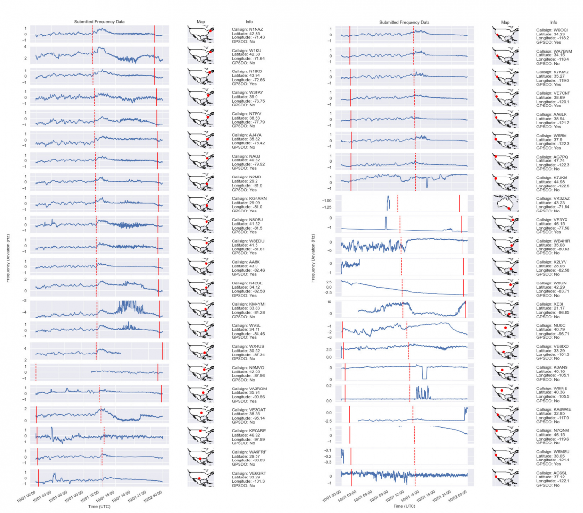
Вы также увидите множество региональных вариаций. Вот график данных, взятых во время Фестиваля частотных измерений. Вы можете прочитать об анализе данных здесь.
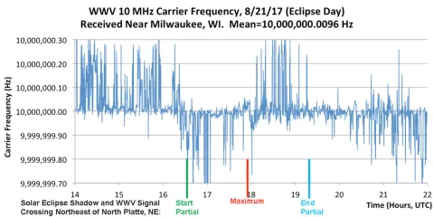
Eclipse and Frequency Measurement Festivals are worldwide citizen science campaigns in which hams and shortwave listeners measure Doppler shift from their home stations, using their regular HF receivers.
Bli med på
Arctic Formørkelsesfestival
Alternate language options:
Engelsk: English
French: Français
Kristina Collins: [email protected]
Vi vil bruke den russiske tidsstandardstasjonen RWM ved 9.996 MHz. Hvis du ikke kan motta den på stasjonen din, kan du prøve 10 MHz WWV eller en annen stasjon fra denne listen. Eksperimenter med radioen din for å se hvilke stasjoner som er enklest å motta.
1) Registrer deg for adresselisten: https://groups.google.com/g/eclipse-festival
2) Følg disse instruksjonene: hamsci.org/doppler-instructions-nb
Bruk Audacity, ikke fldigi.
3) Send inn data her: https://cwru.app.box.com/f/4c75fe21d8f744d980b61916704abd1f
Det vil være en valgfri øvelsesøkt 30. mai for å velge de beste stasjonene for eksperimentet. For å delta, lytt til RWM (4,996 MHz, 9,996 MHz) og WWV (5 MHz, 10 MHz) på radioen din og fullfør undersøkelsen nedenfor. Det er best å ta opp på omtrent samme tid på dagen som formørkelsen (8 am UTC). Hvis mulig, kan du ta et kort opptak med Audacity og laste det opp her.
Interested in translating pages for HamSCI? Email [email protected].
https://hamsci.org/december-2020-eclipse-festival-frequency-measurement-es
Translator: Matt KE8NZR
À propos de HamSCI: https://hamsci.org/about-hamsci-fr
Comment collecter des données sur l'effet Doppler avec votre récepteur radio décamétrique (HF): https://hamsci.org/doppler-instructions-fr
Festival de mesure de fréquence pour l'éclipse de juin 2021: https://hamsci.org/june-2021-eclipse-festival-frequency-measurement-fr
Festival de mesure de fréquence pour l'éclipse de décembre 2021: https://hamsci.org/december-2021-eclipse-festival-frequency-measurement-fr
Translator: Yannick F4IQE
Hulp radioamateurs gevraagd: meet Doppler-verschuiving tijdens eclips: https://www.veron.nl/nieuws/doppler-verschuiving-eclips/
Translator: Erwin PE1CUP
Hvordan samle Doppler-data med din HF-radio: https://hamsci.org/doppler-instructions-nb
Juni 2021 Formørkelsesfestival: https://hamsci.org/june-2021-eclipse-festival-frequency-measurement-nb
Translator: Kristina KD8OXT (Send meg en e-post hvis du ser feil ordene. Jeg lærer fremdeles!)
Dezembro de 2020 Eclipse Festival of Frequency Measurement: https://hamsci.org/december-2020-eclipse-festival-frequency-measurement-pt
Translator: Noilson Caio - Darkwaves
Эффект Допплера: https://www.hamsci.org/doppler-instructions-ru
Translator: Saule Anafinova
6月21日 日全(偏)食高频频率变化测量: https://hamsci.org/june-2020-eclipse-festival-frequency-measurement-cn
French translation of https://hamsci.org/about-hamsci
HamSCI, le Ham Radio Science Citizen Investigation (Enquête citoyenne de Science Radio Amateur), est une plateforme pour faire de la publicité et de la promotion de projets qui sont cohérents avec les objectifs suivants:
HamSCI sert de moyen de favoriser les collaborations entre les chercheurs professionnels et les opérateurs de radio amateur. Il aide à développer et à maintenir des normes et des accords entre toutes les personnes et organisations impliquées.
HamSCI a été lancé par des scientifiques radio amateurs qui étudient la physique de la haute atmosphère et de l'espace. Ces scientifiques ont reconnu que des projets tels que le Reverse Beacon Network, WSPRNet, PSKReporter, DX Cluster, ClubLog, etc. génèrent des ensembles de données volumineuses qui pourraient fournir des observations utiles sur l'ionosphère de la Terre et des systèmes associés. Pour cette raison, l'accent initial de HamSCI est sur ces domaines de recherche. À l'avenir, d'autres chercheurs pourraient rejoindre HamSCI et élargir son champ d'action.
Radiosignaler hjelper oss med å se endringer i ionosfæren. Mange tidsstandardstasjoner har presise bærefrekvenser. Når den virtuelle høyden på ionosfæren stiger og faller, blir frekvensen av HF-signaler påvirket av doppler skift. Med en presis lokaloscillator, som en GPSDO, kan du måle bevegelsen til refleksjonspunktet.
Det er to måter å samle inn data fra lokasjonen din. Du kan ta opp en .CSV-fil for langsiktig datainnsamling, eller ta opp lyd for korte kampanjer (som Eclipse Festival).
Du vil trenge:
Det er mulig å samle inn data uten GPSDO, men målingene dine blir mye bedre med en. Metoden for å koble GPSDO til radioen din vil avhenge av hvilken type radio du har.
Du vil ta opp en stasjon som kan høres fra stasjonen din. Eksemplene nedenfor bruker 10 MHz. Tidsstandardstasjoner: here.
Africa :
Det er ingen HF-tidstasjoner i denne regionen. Bruk RWM eller LOL, PPE.
Asia :
* BPM, China, Shaanxi, Pucheng (sentrale Kina)
2.50 MHz, 5.0 MHz, 10 MHz, 15 MHz (Kraft ukjent)
* HLA, South Korea, Daejeon
5.0 MHz (2 kW)
Europe :
* RWM, Russia, Moscow, Taldom (øst for Europa)
4.996 MHz (10kW), 9.996 MHz (10kW), 14.996 MHz (10kW)
North-America :
* WWV, United States, Colorado, Fort Collins (sentrale USA)
2.50 MHz (2.5 kW), 5.0 MHz (10 kW), 10.0 MHz (10 kW), 15.0 MHz (10 kW), 20 MHz (2,5kW), 25 MHz (2,5kW)
* CHU, Canada, Ontario, Ottawa (sørøst Canada )
3.33 MHz (3 kW), 7.85 MHz (10 kW), 14.67 MHz (3kW)
Oceania :
Det er ingen HF-tidstasjoner i denne regionen.
Bruk WWVH i Hawaii eller BPM i Kina
Pacific Ocean
* WWVH, United States, Hawaii, Kekaha (Pacific)
2.50 MHz (5 kW), 5.0 MHz (10 kW), 10.0 MHz (10 kW), 15.0 MHz (10 kW)
South America
* LOL, Argentina, Buenos Aires
10 MHz (2 kW)
* PPE, Brazil, Rio de Janeiro, Rio de Janeiro
10.0 MHz (1 kW)
* YVTO, Venezuela, Caracas
5.0 MHz (1 kW)
For å velge den beste stasjonen:
1) Bruk nærmeste sender på kontinentet
2) bruk frekvensen med mest effekt (i kW) hvis du kan
3) Vurder følgende:
For kontinentale og nasjonale avstander:
- Om natten: 3MHz til 9 MHz.
- På dagtid: 5 MHz til 16 MHz.
På regionale avstander:
- Om natten: 0.3 MHz til 5 MHz band i Europa, 2 MHz til 6 MHz band i tropene,
- På dagtid: 0.3 MHz til 8 MHz band i Europa, 4 MHz til 12 MHz band i tropene.
Merk: Denne tilnærmingen er for kortvarig datainnsamling, for eksempel formørkelse festivaler. For langsiktig datainnsamling, se Tilnærming 1# ovenfor.

VIKTIG: Hvis du har flere radioer under ett kallesignal, kan du legge til bindestrek og nummer. For eksempel, hvis stasjon W8EDU kjører datainnsamling samtidig på en Flex-radio og en Icom-radio, bør de merke den ene som W8EDU-1 og den andre som W8EDU-2, inkludert en kommentar i metadataene for hver stasjon som forklarer at operatøren kjørte flere stasjoner, og sørg for at metadataene er riktige og fullstendige. Dette vil gjøre det mye lettere å sortere gjennom dataene fra eksperimentet i løpet av analysen.


Du er klar! Hvis du når som helst trenger å starte datainnsamlingen igjen, trykker du på stoppopptaksknappen og gjentar trinn 7 ovenfor.
Når du er klar, bør oppsettet ditt se slik ut:
Du kan plotte dataene dine over tid for å se geofysiske trender. Hvis du mottar et klart signal, bør soloppgangen vises dydelig i frekvensdatene dine.
Du vil se variasjon fra dag til dag. Hvis du plotter data over lang tid, vil du se morgenskiftet endres med lengden på dagen.
En god måte å kontrollere troverdigheten til dataene dine: Be nære venner om å ta data på de samme frekvensene. Dette vil bidra til å skille lokal støy i miljøet ditt fra geofysiske signaler. I plottet nedenfor er alle stasjonene innen 5 km fra hverandre, og de tre stasjonene på toppen har alle GPSDO-er. (Bildekreditt: Wim PA0SLT)
Du vil også se mye regional variasjon. Her er en oversikt over data tatt under den opprinnelige WWV Centennial Festival of Frequency Measurement. Du kan lese om analysen av dataene her.
French translation of https://hamsci.org/december-2021-eclipse-festival-frequency-measurement
du 01 décembre 2021 00:00 au 10 décembre 2021 23:59 UTC
Kristina Collins: [email protected]

Veuillez commencer les mesures avant l'heure de début de la journée et les terminer après l'heure de fin, si possible.
1) Inscrivez-vous sur la liste de diffusion du Festival de l'Eclipse : https://groups.google.com/g/eclipse-festival
2) Collectez des données selon les instructions sur cette page : hamsci.org/doppler-instructions-fr
3)Soumettez vos données ici : https://cwru.app.box.com/f/3300f6a225af40a4b70f653583c9e361
Plus d'informations sur le projet HamSCI :https://hamsci.org/about-hamsci-fr
French translation of https://hamsci.org/june-2021-eclipse-festival-frequency-measurement
du 07 juin 2021 00:00 au 12 juin 2021 23:59 UTC
Kristina Collins: [email protected]
Veuillez commencer les mesures avant l'heure de début de la journée et les terminer après l'heure de fin, si possible.
La principale balise de cette expérience sera la station de signaux horaires russe RWM sur 9.996 MHz. Si vous ne parvenez pas à la recevoir sur votre station de réception radio, veuillez essayer la station américaine WWV sur la fréquence de 10,000 MHz ou une autre station de cette liste. Faites des essais avec votre radio pour voir quelles stations sont les plus faciles à recevoir.
1) Inscrivez-vous sur la liste de diffusion du Festival de l'Eclipse : https://groups.google.com/g/eclipse-festival
2) Collectez des données selon les instructions sur cette page : hamsci.org/doppler-instructions-fr
ATTENTION : Utilisez les instructions sur la collecte de données audio avec le logiciel Audacity, et pas avec le logiciel fldigi.
Si vous avez collecté des données pour le festival Eclipse de décembre 2020, la procédure est très similaire, sauf que la fréquence de l'oscillateur local doit être incluse dans le nom de fichier.
3)Soumettez vos données ici : https://cwru.app.box.com/f/4c75fe21d8f744d980b61916704abd1f
Plus d'informations sur le projet HamSCI :https://hamsci.org/about-hamsci-fr
Il y aura une session pratique facultative le 30 mai pour sélectionner une ou plusieurs stations balises pour l'expérience. Pour participer, veuillez écouter RWM (4,996 MHz, 9,996 MHz) et WWV (5 MHz, 10 MHz) sur votre radio et remplir le sondage ci-dessous. Il est préférable d'enregistrer à peu près à la même heure de la journée que l'éclipse (8 h UTC). Si possible, faites un court enregistrement avec Audacity et téléchargez-le ici.
French translation of https://hamsci.org/doppler-instructions
Les signaux radio offrent une fenêtre sur la couche atmosphérique changeante de l'ionosphère. Les divers signaux de la station de signaux horaires américaine WWV, réfléchis par l'ionosphère, subissent des changements de longueur de trajet à mesure que le profil de densité électronique ionosphérique change. Il en résulte des changements de la fréquence des signaux radio qui est observée aux points de réception. Ceux-ci sont semblables à la montée et à la baisse de niveau d'un sifflet de train qui passe.
Les signaux de la station de radio américaine WWV se reflètent sur l'ionosphère dans cette illustration. La météorologie de l'espace affecte la distance parcourue par un signal avant de changer de direction, et la station réceptrice le détecte comme un changement de fréquence du signal.
La comparaison du signal radio reçu avec un étalon de fréquence local de précision, tel qu'un oscillateur asservi par GPS, permet à un utilisateur de mesurer ces décalages de fréquence induits par l'ionosphère. Cette mesure est préparée et enregistrée avec un logiciel libre (open source). De nombreux ensembles de données enregistrés simultanément à partir de plusieurs emplacements offrent des informations - lorsque ces ensembles de données sont examinés à la fois individuellement et collectivement - sur l'ionosphère au moment où les données sont prises. Ces informations comprennent les mouvements des perturbations ionosphériques en déplacement et d'autres phénomènes importants à différentes échelles.
Vous pouvez en savoir plus sur le fonctionnement de ces mesures ici.
Il existe deux façons de collecter des données de l'effet Doppler-Fizeau à partir de votre position géographique (QTH). La première consiste à collecter des données au format tableur .CSV à l'aide d'un programme d'analyse de fréquence - c'est le mieux pour la collecte de données à long terme. L'autre consiste à collecter des fichiers audio, ce qui n'est recommandé que pour des expériences à court terme telles que les festivals d'éclipse.
Vous aurez besoin de:
La méthode de connexion du GPSDO à votre récepteur radio dépendra du type de radio dont vous disposez.
Il est possible de collecter des données sans GPSDO, mais vos mesures seront bien meilleures en utilisant un. Bien que vous puissiez voir les tendances dans vos données, vous ne serez pas en mesure de faire une estimation quantitative de la hauteur de la couche. Comme le montre ce graphique de Steve Cerwin WA5FRF, une petite erreur dans la fréquence de votre oscillateur local se traduit par une grande erreur au fil du temps lors de l'estimation de la hauteur de la couche:
Vous voudrez enregistrer une fréquence de balise qui peut être entendue à partir de votre station de réception (récepteur radio). Les exemples sur cette page utilisent la fréquence radio avec un signal horaire de référence à 10 MHz. Vous pouvez trouver une liste des stations de signaux horaires de référence ici.
Stations de signal horaire radio dans le monde avec des transmissions à ondes courtes que vous pouvez utiliser pour les mesures de fréquences pendant le festival de l'Eclipse (Eclipse Festival of Frequency Measurement) :
Afrique :
Aucune station avec des transmissions en ondes courtes.
Pays africains de l'hémisphère nord: utiliser RWM en Russie
Pays africains de l'hémisphère sud: essayez de recevoir l'une des stations de signal horaire d'Amérique du Sud, Sinon, utilisez RWM en Russie
Asie :
* BPM, Chine, Shaanxi, Pucheng (Chine centrale)
2.50 MHz, 5.0 MHz, 10 MHz, 15 MHz (puissance en kW inconnue pour chaque fréquence)
* HLA, Corée du Sud, Daejeon
5.0 MHz (2 kW)
Europe :
* RWM, Russie, Moscou, Taldom (est de l'Europe)
4.996 MHz (10kW), 9.996 MHz (10kW), 14.996 MHz (10kW)
Amérique du nord :
* WWV, États-Unis, Colorado, près de Fort Collins (centre des États-Unis d'Amérique)
2.50 MHz (2.5 kW), 5.0 MHz (10 kW), 10.0 MHz (10 kW), 15.0 MHz (10 kW), 20 MHz (2,5kW), 25 MHz (2,5kW)
* CHU, Canada, Ontario, Ottawa (dans le sud-est du Canada)
3.33 MHz (3 kW), 7.85 MHz (10 kW), 14.67 MHz (3kW)
Océanie :
Aucune station avec des transmissions en ondes courtes.
Utilisez WWVH à Hawaï ou BPM en Chine
Océan Pacifique
* WWVH, États-Unis, Hawaï, Kekaha (au centre de l'océan Pacifique nord)
2.50 MHz (5 kW), 5.0 MHz (10 kW), 10.0 MHz (10 kW), 15.0 MHz (10 kW)
Amérique du sud
* LOL, Argentine, Buenos Aires
10 MHz (2 kW)
* PPE, Brésil, Rio de Janeiro, Rio de Janeiro
10.0 MHz (1 kW)
* YVTO, Vénézuéla, Caracas
5.0 MHz (1 kW)
Recommandations pour choisir la meilleure station de radio
1) Utilisez l'émetteur le plus proche sur votre continent
2) utilisez la fréquence avec le plus de puissance (en kW) si vous le pouvez
3) pour choisir la fréquence de réception, essayez:
Pour les radiocommunications continentales et nationales, nous pouvons résumer
- la nuit: bandes de 3 MHz à 9 MHz,
- de jour: bandes de 5 MHz à 16 MHz.
Pour les radiocommunications régionales et départementales, nous pouvons résumer
- la nuit: bande 0,3 MHz à 5 MHz en Europe, bande 2 MHz à 6 MHz sous les tropiques,
- de jour: bande 0,3 MHz à 8 MHz en Europe, bande 4 MHz à 12 MHz sous les tropiques.
Informations plus détaillées par bande de fréquence : voir "Propagation en fonction de la fréquence" dans l'article Propagation en haute fréquence sur Wikipedia.
Nous vous demandons d'utiliser spécifiquement le logiciel libre (open-source) fldigi-4.1.13 ou une version ultérieure. Son mode «analyse de fréquence (frequency analysis)» génère quotidiennement des fichiers d'écarts/déviations de fréquence, qui sont automatiquement nommés «analysis_ (date) .csv». Ceux-ci seront créés dans le répertoire /fldigi/temp /, ou .fldigi/temp/, ou quelque chose d'équivalent. Vous devez utiliser une version récente de fldigi, sinon vos données seront écrasées.
Remarque: Cette méthode est pour la collecte de données à court terme, comme pendant les festivals d'éclipse. Pour la collecte de données à long terme, nous vous recommandons d'utiliser le logiciel fldigi suivant la procédure décrite ci-dessus.
1) Connectez votre récepteur radio à la carte son de votre ordinateur.
Si vous contrôlez votre récepteur radio via les logiciels fldigi ou flrig, vous devez déjà savoir le faire. Les instructions varient selon les récepteurs radio. Si vous avez besoin d'une carte son USB, nous vous recommandons celle-ci: https://www.amazon.fr/gp/product/B00IRVQ0F8/ref=ppx_yo_dt_b_asin_title_o03_s00
2) Téléchargez Audacity.
Audacity est un logiciel libre (open source) réputé pour l'enregistrement audio. Vous pouvez le télécharger ici: https://www.audacityteam.org/download/
Si vous l'utilisez dans une langue autre que l'anglais, vous pouvez la choisir en utilisant le menu Edit > Preferences > Interface (dans le panneau gauche de la nouvelle fenêtre) > dans la section "Display", pour le champ "Language", sélectionnez "Français" dans la liste déroulante à la place de "English".
3) Configurez les métadonnées Audacity.
Téléchargez ce modèle XML et notez le répertoire dans lequel le téléchargement dépose le fichier: EclipseTags.xml
Sous le menu "Edition > Métadonnées..." (en anglais menu "Edit>Metadata..."), cliquez sur le bouton "Charger" et sélectionnez le fichier puis cliquez sur le bouton "Ouvrir", puis modifiez-le pour l'adapter à votre station. (Vous pouvez également ajouter des métadonnées manuellement en utilisant la liste ci-dessous.)

Dans Audacity, aller dans Modifier> Métadonnées (Edit>Metadata) et remplissez les champs de métadonnées suivants:
ATTENTION : NE PAS MODIFIER LES TEXTES DE LA COLONNE "BALISE" AFIN DE PERMETTRE LE TRAITEMENT AUTOMATISE DES DONNEES PAR LA SUITE
Ajoutez et remplissez les champs de métadonnées suivants en anglais.
IMPORTANT: Si vous avez plusieurs récepteurs radios qui collectent des données simultanément sous un seul indicatif, ajoutez un trait d'union et un numéro de station pour chaque station dans tous les cas ailleurs où vous allez devoir utiliser aussi l'indicatif. Par exemple, si la station W8EDU effectue la collecte de données simultanément sur un récepteur radio Flex et un récepteur radio Icom, ces données doivent être étiquetées l'une comme W8EDU-1 et l'autre comme W8EDU-2. Veuillez inclure un commentaire dans les métadonnées de chaque station expliquant que l'opérateur a recueilli des données à partir de plusieurs stations et assurez-vous que les métadonnées sont correctes et complètes. Cela rendra beaucoup plus facile le tri des données de l'expérience scientifique pendant la phase d'analyse.
Appuyez sur le bouton "Sauvegarder" puis le bouton "Enregistrer" et enregistrez le fichier XML, puis appuyez sur le bouton "Réglages par défaut".
Cochez la case "Ne plus montrer cet avertissement pendant un export audio", puis cliquez sur "Valider".
4) Paramétrage des préférences d'enregistrement.
Ouvrez l'onglet Enregistrement dans le menu Préférences (menu Edition> Préférences... > Enregistrement (dans le panneau gauche)). Dans la section "Options", décochez l'option "Doublage : Lire les autres pistes pendant l'enregistrement d'une nouvelle (overclub)" et cochez "Enregistrer sur une nouvelle piste" et "Détecter les désynchronisations".
Dans la section "Nommer les pistes nouvellement enregistrées", cochez l'option "Nom de la piste personnalisé", entrez votre indicatif dans le champ en face de ""Nom de la piste personnalisé"", puis un seul trait de soulignement, puis la lettre correspondant à votre fuseau horaire dans cette liste: [https://fr.wikipedia.org/wiki/Liste_des_zones_horaires_militaires]
Par exemple, la station W8EDU est en heure normale de l'Est américain (EST - Eastern Standard Time) (UTC - 05:00), ce qui correspond à la lettre R, donc la valeur correcte dans le champ "Nom de la piste personnalisé" commencera avec "W8EDU_R_". (Si vous êtes dans un fuseau horaire fractionnaire, utilisez la lettre J; cela marquera votre jeu de données pour un traitement manuel en fonction de votre emplacement.)
Ajoutez la fréquence de l'oscillateur local de votre récepteur radio. Par exemple, si la station de réception W8EDU est réglé sur la fréquence 9,999 MHz pour écouter la station de signaux horaires américaine WWV à 10 MHz , le champ de nom de piste personnalisé doit indiquer "W8EDU_R_9999kHz_". Si la station de réception W8EDU est réglé sur 9,995 MHz pour écouter la station de signaux horaires russe RWM à 9,996 MHz, le champ de nom de piste personnalisé doit indiquer "W8EDU_R_9995kHz_". Cette instruction a été ajoutée pour le festival de l'Eclipse de juin 2021 et n'apparaît pas actuellement dans les captures d'écran ci-dessous.
Assurez-vous que les cases "Date système" et "Heure système" sont également cochées. Lorsque vous avez terminé, la fenêtre devrait ressembler à ceci:

Sous "Qualité" dans le panneau gauche, définissez "Format d'échantillonnage par défaut" sur 16 bits. Réglez "fréquence d'échantillonnage par défaut" à 8000 Hz (sauf si votre récepteur requiert une fréquence plus élevée, comme décrit à l'étape 2 ci-dessus).
Allez dans "Périphériques" dans le menu Préférences et assurez-vous que vous enregistrez à partir de votre récepteur radio, par opposition au microphone de votre ordinateur ou d'une autre source.
Une fois terminé, cliquez sur OK.
5) Définissez les paramètres d'enregistrement et effectuez un test d'enregistrement.
Réglez votre enregistrement sur Mono (1 canal) dans le menu déroulant au milieu de la barre d'outils supérieure.
Assurez-vous que la fréquence de votre projet est réglée sur 8000 Hz dans le menu déroulant dans le coin inférieur gauche de l'écran.
Réglez votre entrée audio sur la carte son connectée à votre récepteur radio. Les noms des appareils varieront. Vous devrez peut-être faire des essais pour vous assurer que la source à partir de laquelle vous enregistrez est la bonne.
Appuyez sur le bouton d'enregistrement ⬤; vous devriez voir la première piste commencer l'enregistrement, avec le nom de piste et l'horodatage corrects. Si le nom de la piste n'est pas correct, essayez de redémarrer votre ordinateur et d'enregistrer à nouveau.
Appuyez sur stop ⏹️, puis enregistrez ⬤ à nouveau. Cette fois, vous devriez voir apparaître une deuxième piste. Le nom de chaque piste correspondra à son heure de début.
Notez l'"Espace disque restant pour l'enregistrement" en bas de votre écran. Une semaine d'enregistrement dure 168 heures, vous devrez donc peut-être suspendre et redémarrer la collecte de données pendant l'expérience. L'estimation peut également ne pas être entièrement exacte. Consultez la documentation d'Audacity sur la durée d'enregistrement ici.
6) Enregistrez le projet.
Assurez-vous d'arrêter ⏹️ l'enregistrement avant de continuer.
Enregistrez le projet (Fich1ier> Enregistrer). Cela permettra à l'ordinateur de conserver vos paramètres. Vous pouvez voir une fenêtre vous demandant si vous souhaitez enregistrer le projet même s'il ne contient aucune piste: cliquez sur OK.
7) Assurez-vous que vos fichiers WAV sont correctement enregistrés.
Créez un répertoire dans lequel enregistrer vos fichiers selon la convention suivante: "<Indicatif>_Eclipse_Dec2020". Par exemple: W8EDU_Eclipse_Dec2020. (Si vous exécutez la collecte de données simultanément sur plusieurs rcepteurs radios, utilisez l'indincatif avec trait d'union décrit à l'étape 3.)
Allez dans le menu "Fichier> Exporter> Export multiple...". Sélectionnez le répertoire dans lequel vous souhaitez enregistrer vos fichiers. Sous "Renommer le fichier", assurez-vous que l'option "Selon le marqueur ou le nom de la piste" est sélectionnée.
Cliquez sur "Exporter". Vous devriez avoir une boîte de dialogue confirmant que chaque piste a été enregistrée dans son propre fichier WAV. (Remarque: si vos fichiers sont trop volumineux pour être exportés, consultez la FAQ ci-dessous.)

Lorsque cela est fait, vous pouvez supprimer vos pistes de test en cliquant sur le X dans le coin supérieur gauche de la piste.
Lorsque vous ouvrez le répertoire, vous devriez voir les métadonnées de l'artiste et de l'album. Confirmez que vos noms de fichiers sont au format correct: "W8EDU_R_9.999MHz_2020-10-23_22-36-18.wav"., Par exemple.
Vous devriez enregistrer vos données sur un lecteur disposant d'au moins 10 Go d'espace libre. Si vous exécutez MS Windows, allez dans votre répertoire de données et activez la compression: Propriétés -> Général -> Avancé -> Compresser le contenu pour économiser de l'espace disque. (Voir la capture d'écran ci-dessous).
8) Facultatif: étalonnez la sortie audio pour l'enregistrement de fichier .WAV
Nous sommes intéressés à collecter des données d'amplitude lorsque cela est possible; vous pouvez en savoir plus ici. Si votre radio dispose d'un circuit de contrôle automatique de gain (AGC ou CAG) qui peut être désactivé et d'un contrôle de gain RF séparé, vous pouvez aussi collecter des données d'amplitude. Cependant, il ne suffit pas d'éteindre l'AGC ou CAG; vous devez régler le gain RF à un niveau approprié. Sinon, le niveau audio sera presque constant quelle que soit la force du signal, et les données pourraient être compromises. Une fois que l'AGC ou CAG est désactivé, la commande de gain RF du récepteur doit être réglée de sorte que le niveau audio donne des amplitudes mesurables qui ne vont jamais au maximum de l'échelle (ou à pleine échelle/niveau maximum), s'écrêtent ou se limitent. Cela nécessitera des tests préliminaires pour être sûr que la force maximale du signal ne saturera pas l'entrée de la carte son. Si votre récepteur radio ne répond pas à ces exigences, passez à l'étape 9 ci-dessous.
Voici une méthode pour configurer le récepteur:
Lorsque vous soumettez votre collecte de données ci-dessous, assurez-vous de confirmer que vous avez bien exécuté cette procédure.
9) Tout est prêt!
Vous devriez maintenant être prêt à collecter des données! Si vous devez redémarrer la collecte de données à tout moment, appuyez sur le bouton Arrêter l'enregistrement et répétez l'étape 7 ci-dessus.
Une fois que vous êtes prêt, votre configuration devrait ressembler à ceci:
Vous pouvez faire le tracé de vos données au fil du temps pour voir les tendances géophysiques. Si vous recevez un signal clair, le lever du soleil devrait apparaître clairement dans vos données de fréquence.
Vous verrez des variations au jour le jour. Si vous faites le tracé des données sur une longue période, vous verrez le décalage de la pointe du matin avec l'évolution de la durée de la journée.
Un bon moyen de vérifier la fidélité de vos données: recrutez des amis à proximité de votre domicile ou site pour prendre des données sur les mêmes fréquences. Cela aidera à séparer le bruit local de votre environnement des signaux de nature géophysique. Dans le graphique ci-dessous, toutes les stations sont à moins de 5 km l'une de l'autre et les trois stations du haut ont toutes des GPSDO. (Crédit de l'image: Wim PA0SLT)
Vous verrez également beaucoup de variations régionales. Voici un graphique des données prises lors du premier "Festival of Frequency Measurement" (Festival de mesure de fréquence). Vous pouvez en savoir plus sur l'analyse des données ici.
Q: Pour quel usage ces données seront-elles utilisées?
R: Ces données seront analysées par les membres de l'organisation HamSCI. Les données et les résultats seront rendus publics, comme nous l'avons fait pour le premier "Festival of Frequency Measurement" (Festival de mesure de fréquence).
Q: Si j'ai du mal à faire fonctionner la collecte de données, pouvez-vous m'aider?
R: Oui. Envoyez un courriel à [email protected] et nous vous aiderons à configurer votre récepteur radio.
Q: Puis-je utiliser un programme autre qu'Audacity pour effectuer mes mesures?
R: Oui, mais nous ne pouvons pas fournir d'assistance pour d'autres programmes. Cependant, nous aimons aussi Spectrum Lab.
Q: Comment puis-je vérifier les métadonnées de mes fichiers WAV?
R: La plupart des outils de métadonnées n'afficheront pas les champs non standard que nous avons ajoutés, mais vous pouvez utiliser mediainfo si vous souhaitez les voir. Il a également une belle interface en ligne de commande.
Q: Pouvez-vous toujours utiliser mes données si je ne peux pas enregistrer pendant toute la période?
R: Plus de données, c'est toujours mieux, mais si vous devez reprendre votre radio pour une partie de l'événement (par exemple, pour gérer un réseau de trafic) ou subir une interruption de données, alors nous sommes toujours intéressés par vos données. Assurez-vous simplement d'arrêter l'enregistrement avant de refaire le réglage en fréquence de votre récepteur radio. Et de revenir à 9,999 MHz avant de le redémarrer lorsque vous êtes prêt à reprendre la collecte de données et de nous laisser une note d'information lorsque vous la soumettrez.
Q: Accepterez-vous d'autres formats de données?
R: Oui, bien que nous ne puissions pas garantir que nous pourrons les utiliser.
Q: Je peux collecter des données pour l'expérience, mais ma connexion Internet est si lente que je ne pourrai pas vous les déposer sur le serveur. Puis-je les soumettre d'une autre manière?
R: Oui! Envoyez-moi un courriel à [email protected] et je vous enverrai une clé USB.
Q: Audacity m'indique que mon enregistrement est trop volumineux pour être exporté sous forme de fichier WAV. Pourquoi cela se produit-il et que puis-je faire ?
R: Les fichiers WAV sont limités à 4 Go parce que la taille du fichier est indiquée dans l'en-tête par un entier 32 bits non signé. Audacity vous donnera une autre chance d'exporter. Sélectionnez "Autres fichiers non compressés", puis sous "En-tête", sélectionnez "WAV (NIST/Sphere)". Cela utilisera un format d'en-tête différent, mais vos données doivent être les mêmes et peuvent être déposées sur le serveur tant qu'elles sont d'une taille inférieure à 32 Go.

Q: Je suis en mesure de configurer une station pour collecter des données sur le long terme. Cela vous intéresserait-il ?
R: Oui! Envoyez un courriel à [email protected] pour en discuter davantage.
The original Grape 1 WWV Doppler received was designed and components available between 2019 and late 2022. It has since been superseded by a new version with greater frequency range and better performance. See the Grape 1 page for complete details.
For complete information on how to build and operate the Grape V1.11, please refer to this paper: https://doi.org/10.1016/j.ohx.2022.e00289
For information on how to access, visualize and interpret data collected by Grape V1.11 Doppler receivers, please refer to this preprint: https://doi.org/10.5194/essd-2022-303
The following is archival information: This web page may be used by those who built the grape1 receivers who need help with details of construction and use of the Grape 1. In order to get an answer to a particular question, please email your question to Jim at [email protected] (at a later date we will have a question submission form on this page). A good introduction may be downloaded at Intro Gen 1 Grape_Ver_1.1.pdf. The presentation may be previewed below. We encourage you to download this and read it now. Then see below for the lists of parts you will need.
We want you to have a good time building and enjoying your Grape 1 receiver, and we need your valuable contributions to the project, but we also need to let you know of certain considerations when you are contemplating your build.
The Purpose
The receiver is a special-purpose receiver designed to record certain data you will measure from your location and submit to the HamSCI organization. This data will provide useful guidance for the scientists and engineers leading the project, and will help guide future stages of the project.
It has been said that the sound of progress is not “Eureka,” but rather is, “That’s funny; why did it do that?” Research is often a “messier” process than it is portrayed in books. When you start a research project, you don’t have all the answers to the questions you have posed – else why would you need to do research? This leads at times to going in a certain direction, only to find out that you hadn’t chosen the optimum direction for investigation, so you back out and partially redirect your efforts. You sometimes discover that the answers you want are available, but you need equipment that is more sensitive, has higher resolution, needs a better signal-to-noise ratio, or whatever. Or sometimes you discover that you were asking questions that were not quite the ones you should be asking in order to accomplish your goal. In this project, we benefit from a lot of previous research on the ionosphere, and we are plowing forward to get answers to remaining questions, such as how the ionosphere interacts with electromagnetic forces from outside of the earth (“space weather”).
Grape 1 is a step leading to the Grape 2, a more capable receiver, and eventually to the Tangerine SDR, a general purpose SDR with added capabilities that make it useful for this research. It will eventually be a modular SDR, with whatever capabilities prove useful. Grape is NOT a general purpose software defined receiver (SDR). It will not allow you to listen on the bands, because it is designed for specific data collection applications.
The Grape 1 is incomplete without a GPSDO (GPS Disciplined Oscillator) that can tune to the frequencies of 2.499, 4.999, and 9.999 MHz, each 1 kHz below a frequency used by radio stations WWV and WWVB, as well as several other time standard stations around the world. The Grape can also be used to tune to CHU, the Canadian standards stations. It needs a Raspberry PI processor with certain support circuits and special-purpose software, which software will be provided. Elsewhere on this web site you’ll find a list of what is needed.
The GPSDO acts as a very stable local oscillator (LO) for the receiver, with WWV (or another station on the same frequency, or CHU on its frequencies) as the carrier. The 1 kHz IF signal that results from mixing the LO and carrier is filtered and either recorded or further processed to yield a signal that contains propagation data of interest. For example, we can see in very small variations in the LO frequency, the effect of Doppler shift as the ionosphere goes up and down with the time of the day. Note that we cannot measure the ionospheres’s height, but only the change in height.
The part of the Grape 1 that must be assembled is the mixer and filter. The printed circuit board (PCB) you assemble supplies an analog audio signal for the Raspberry PI computer, which records the desired data and/or sends it to a server that acts as a repository for the data. It is then analyzed by project scientists to glean data needed to define certain reactions of the ionosphere.
The board that must be assembled uses very tiny surface mounted components in order to keep it small. The PCB itself is purchased from OSH Park, a custom PCB house, and the parts that go on it are purchased from Digikey or another component vendor. Other parts such as the Raspberry PI and sound interface can be purchased from Amazon or another vendor. You should know that the board, though small, is very dense and the components are VERY small. It is possible to assemble the PCB by hand, but it is somewhat tedious. Assembly requires patience and persistence. It is not a project for a beginner. You will need a good bit of soldering skill, and access to the right tools for working with surface mount components. These tools include a soldering iron with a very small tip, preferably temperature controlled, small diameter wire solder, a lighted magnifier or a low powered microscope, and several pair of tweezers.
Assembly directions are and will continue to be sparse and will assume prior experience and skill. There are no step-by-step assembly instructions. We have organized this help group to help guide you as you have questions. The members of the group are all volunteers with a good bit of experience, but we have never seen this project before either, because the whole project is new. You will be able to email your questions related to the assembly of the mixer/filter board, and using the completed project. We will answer you by email. Please allow a reasonable amount of time for an answer, as we are all volunteers ourselves, with the usual responsibilities and pressures, doing this as a labor of love. Unfortunately we are not able to diagnose problems with your PCB, and we are not able to repair PCBs that don’t work.
As we accumulate knowledge of the questions people have, we will assemble that knowledge into an FAQ section, which will be posted here, of course without any identifying information as to who raised the question.
First some hints for building the board, then the parts lists
- Use a pair of tweezers to hold the parts, and don't squeeze them too much, as holding it tightly will just give the part more energy to fly off when (not if) it slips out of your tweezers.
- The easiest way to solder parts on the PCB is to put solder on one pad then mount the part, soldering that lead first, followed by soldering other pins.
- We found it helpful to do your assembly in a large cookie sheet with low sides; the parts have a way of escaping from your tweezers, and the cookie sheet prevented the loss of many a part.
- You will need a very small tip on your soldering iron, and the soldering iron is preferably temperature controlled. We used the Hakko FX888D-23BY Digital Soldering Station and we like the Hakko T18-BR02 tip, but other irons and tips are just as good. Of course other places also sell these. Keep the tip VERY clean.
- The mixer IC can be put on the board two ways, the right way and the wrong way, rotated 180 degrees. There is a small white circle on the PCB near pin 1. The package may only identify the orientation by a slight slant on the edge of the package. It should be oriented with the slant toward the outside of the PCB. Looking from the top of the IC, the pin numbers progress counter-clockwise (clockwise if you look from the bottom of the IC), and pin 1 is on the side with the slant.
The following has already been made available to participants, but is presented here as a service for any new builders.
The parts list, with Digikey part numbers is below. John, N8OBJ, was kind enough to prepare a list for you. Of course you don't have to buy your parts from Digikey, just make sure that the parts have the same electrical and mechanical specifications. We STRONGLY suggest purchasing extra parts, as they have a habit of jumping from your tweezers and sometimes never being seen again.
| QTY | REF. DSGNS. | Digikey # |
| 6 | C5+C8+C9+C12+C17+C18 | 399-8000-1-ND |
| 3 | C3+C4+C6 | 399-17616-1-ND |
| 1 | C7 | 732-8077-1-ND |
| 1 | C11 | 732-7678-1-ND |
| 4 | C13+C14+C16+C19 | 445-5985-1-ND |
| 1 | C1 | 478-1364-1-ND |
| 1 | C10 | 732-8066-1-ND |
| 1 | C15 | 732-8068-1-ND |
| 1 | C2 | 732-8070-1-ND |
| 1 | R3 | P49.9CCT-ND |
| 1 | R2 | P402CCT-ND |
| 3 | R1+R9+R10 | P1.00KCCT-ND |
| 2 | R4+R5 | 311-10KARCT-ND |
| 1 | R6 | 541-121KCCT-ND |
| 2 | R7+R8 | 541-240KCCT-ND |
| 1 | D2 | 1N4001RLGOSCT-ND |
| 1 | D1 | ESD7L5.0DT5GOSCT-ND |
| 2 | L1+L4 | 490-6604-1-ND |
| 1 | L3 | 490-16851-1-ND |
| 1 | L5 | 490-11672-1-ND |
| 1 | L2 | 490-12091-1-ND |
| 1 | PWR | 754-2118-1-ND |
| 1 | IC3 | LT1761IS5-5#TRMPBFCT-ND |
| 1 | U1 | LT6202CS5#TRMPBFCT-ND |
| 1 | IC1 | 568-5045-1-ND |
| 2 | ANT+LO | CON-SMA-EDGE-S-ND |
| 1 | FREQ | 609-3234-ND |
| 1 | JMP1 | S9337-ND |
You will need some other things of course, and John has prepared a list of them too.
| # | Description | Source |
| 1 | Grape Gen 1 Receiver board assembled by you | https://oshpark.com/shared_projects?utf8=%E2%9C%93&search%5Bquery%5D=WWV_Radio_V1_11&button=&search%5Bfilters%5D%5Bpcb_layers%5D%5Btwo_layer%5D=1&search%5Bfilters%5D%5Bpcb_layers%5D%5Bfour_layer%5D=1&records_date_sort=desc&records_per_page=20 or go to oshpark.com, at the bottom of the page find CONNECT then SHARED PRODUCTS, then search for WWV_Radio_V1_11 |
| 2 | RaspberryPi 4B w/4GB memory | https://www.amazon.com/gp/product/B07TC2BK1X/ref=ppx_yo_dt_b_asin_title_o00_s00?ie=UTF8&psc=1 |
| 3 | High Endurance 64GB uSD Card | https://www.amazon.com/gp/product/B07B9KTLJZ/ref=ppx_yo_dt_b_asin_title_o02_s00?ie=UTF8&psc=1 |
| 4 | Custom OS Image with all software installed (compressed) | https://drive.google.com/drive/folders/1YE5UjQknnhuRUq4Y86czhxbIwzUWbgbn?usp=sharing |
| 5 | Case w/fan and 4 heatsinks | https://www.amazon.com/gp/product/B07W5VQYG9/ref=ppx_yo_dt_b_asin_title_o01_s00?ie=UTF8&psc=1 |
| 6 | Sabrent USB sound adapter | https://www.amazon.com/gp/product/B00IRVQ0F8/ref=ppx_yo_dt_b_asin_title_o00_s00?ie=UTF8&psc=1 |
| 7 | Leo Bodnar GPSDO unit | http://www.leobodnar.com/shop/index.php?main_page=product_info&cPath=107&products_id=301 |
| 8 | 4” SMA-M to SMA-M cable | https://www.amazon.com/gp/product/B072FS4WMK/ref=ppx_yo_dt_b_asin_title_o04_s01?ie=UTF8&psc=1 |
| 9 | 4” SMA-M to SO-239 cable | https://www.amazon.com/gp/product/B00COW5E3A/ref=ppx_yo_dt_b_asin_title_o06_s00?ie=UTF8&psc=1 |
| 10 | 1/8” Stereo cable (~10 – 12 inches) | https://www.amazon.com/gp/product/B0047741BG/ref=ppx_yo_dt_b_asin_title_o03_s00?ie=UTF8&psc=1 |
| 11 | A lot of patience and motivation... |
From within you. Ain't coming from anywhere else |
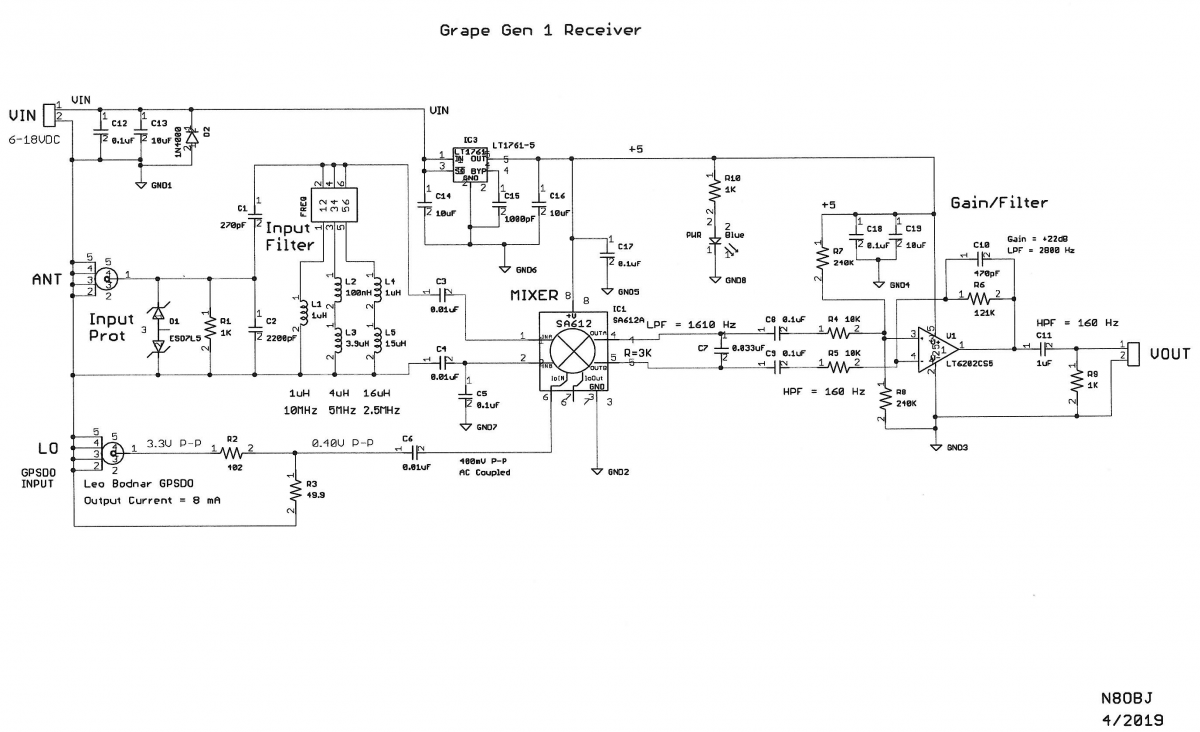
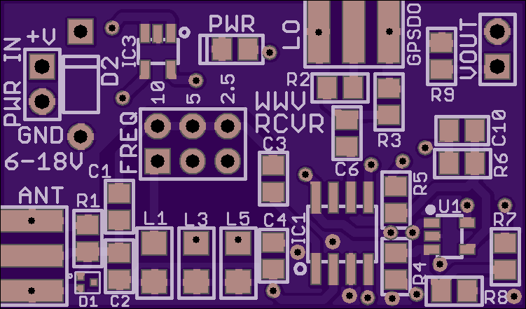
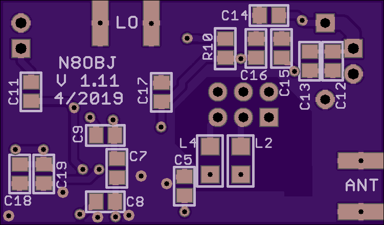
Please upload your .CSV and (optionally) .PNG files here at your leisure. Real-time uploading is in development.
Data can be found at www.doi.org/10.5281/zenodo.6622111. For visualization tools, please refer to https://essd.copernicus.org/preprints/essd-2022-303/.
We are still organizing our data storage systems, but here are some long-term datasets to consult. Please contact [email protected] if you would like to use these data in a publication.
The concept of the HamSCI Radiosport League was developed during the HamSCI 2021 workshop.
Solar Eclipse QSO Party, Golden Ears Project, Festival of Frequency Measurement
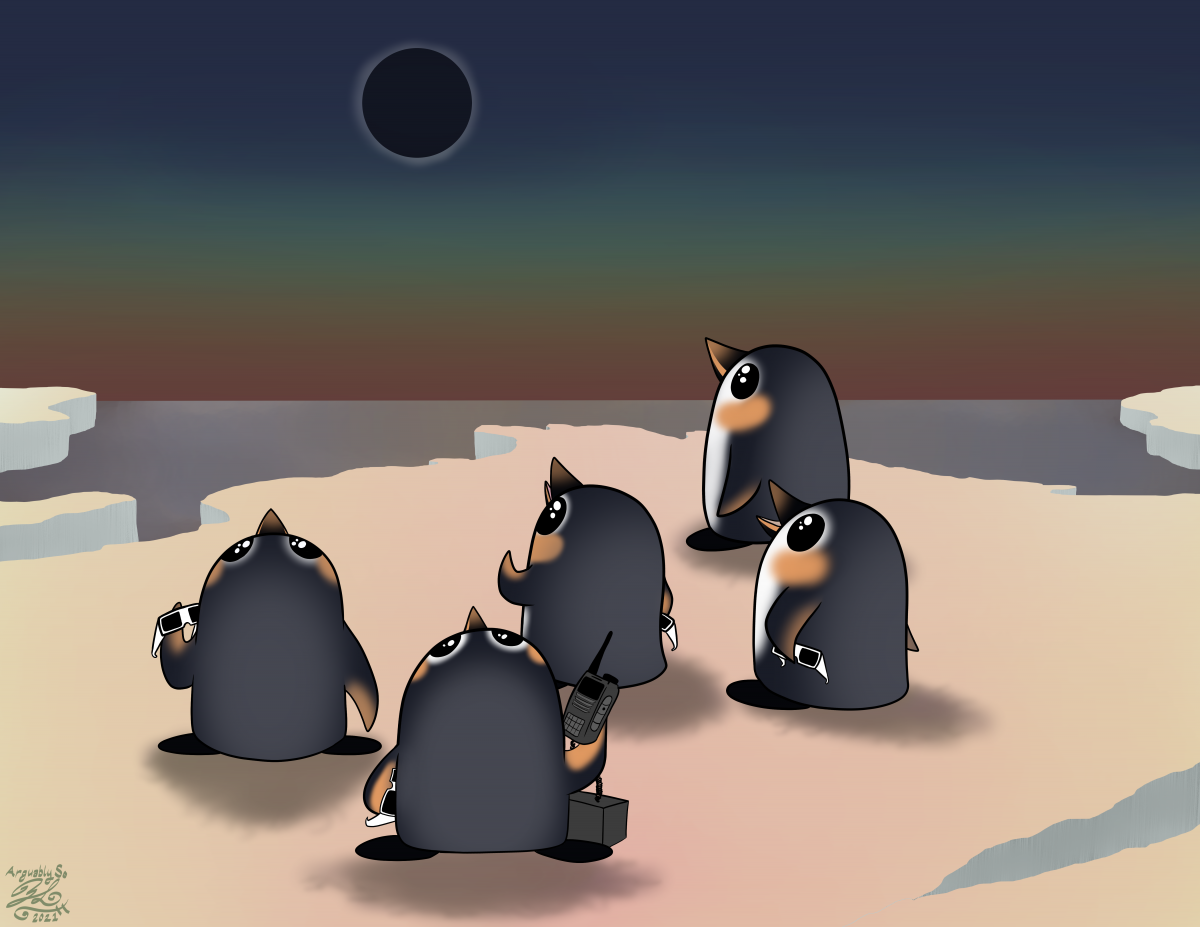
Kristina Collins: [email protected]
______________________________________________________________________________________________________________
If you would like to help test an existing project, look at the project list below and contact the lead for a project that looks interesting. Project leads are responsible for maintaining a list of software testers.
If you would like to develop a project, email [email protected] with the subject line "Eclipse Festival Software Project." Include the following information:
A list of software projects will go here.
Project Description: A Fall 2021 senior project at CWRU to replace Audacity for metadata recording.
Development Team: Zachary Kadish  , Martin Bui, Daniel Warner, Shivvanandh Mohan
Testing Team: TBD
Current Status: In development; will be seeking testers shortly.
Project URL: www.hamsci.org/snash

Project Description: A GNU Radio flowgraph for measuring Doppler with your SDR.
Development Team: Marcus Leech
Current Status: Available for use. (If you record I/Q data, please post it to Zenodo or upload it below in a zipped file with a text document describing your setup.)
Project URL: https://github.com/ccera-astro/wwv_doppler
Contact Information: https://chat.gnuradio.org/#/room/#wwv:gnuradio.org
Project Description: A GNU Radio flowgraph for measuring Doppler from audio using the PLL Detection function, as a flexible alternative to fldigi.
Developers and Testers: K0ZEL, KD8OXT, PE1MJA
Current Status: Testing existing code. Next steps: CSV logging, sideband detection.
Project URL: https://zenodo.org/record/5725910
Contact Information: https://chat.gnuradio.org/#/room/#wwv:gnuradio.org
Project Description: A special test signal is being transmitted on WWV/H to characterize the transmitters. The current version of the signal will run through January 30.
Development Team: WWV/H Scientific Modulation Working Group
Current Status: Looking for ways to compare signal recordings (https://zenodo.org/record/5715673) to the ground truth (https://zenodo.org/record/5602094), and to develop citizen science experiments using the test recording.
Project URL: https://hamsci.org/wwv
Contact Information: [email protected] or https://chat.gnuradio.org/#/room/#wwv:gnuradio.org
Project Description: This repository contains a brief analysis result and the scripts (of shell, R, awk, etc.) used to obtain the frequency/amplitude data from the daily recorded output of Grape 1 (and any receiver applicable with 8kHz WAV file). I've been developing this set of scripts since the last year's December 2020 Festival. You need to specify the WAV filename, starting time (in UNIX/POSIX epoch), and pitch difference in ppm (which can be measured by how much *actual* time was spent for 86400*8000 samples of the WAV file (supposed to be one day if the recording timing has no error).
Development Team: Kenji Rikitake, JJ1BDX
Current Status: So far successfully made analysis of the data during 1 to 6 December 2021. The results are given in the own graphs and fldigi-compatible daily analysis data, as well as the text value files of frequency and amplitude information.
Project URL: https://github.com/jj1bdx/hamsci-202112-freqdata
Contact Information: Please use GitHub issues at https://github.com/jj1bdx/hamsci-202112-freqdata.
If you are interested in working on a software project, these tools will be of use to you:
GNU Radio is a free, open-source platform for digital signal processing. It will be used in several of the software projects.
Installation Guides: https://wiki.gnuradio.org/index.php/InstallingGR
Tutorials: https://wiki.gnuradio.org/index.php/Tutorials
Chat Channels: chat.gnuradio.org
Zenodo is a FAIR Data repository which can be used to store referenceable files. Eclipse Festival participants are encouraged to submit datasets to Zenodo and include them in the HamSCI community page there, so that they may be easily listed and referenced later.
______________________________________________________________________________________________________________
1) Sign up on the Eclipse Festival mailing list: https://groups.google.com/g/eclipse-festival
2) Collect data according to the instructions on this page: hamsci.org/doppler-instructions
3) Upload your data to Zenodo or submit it via the link below.
4) Fill out the exit survey at the bottom of this page.
______________________________________________________________________________________________________________
Why this shift in focus?
While previous Eclipse Festivals have focused on crowdsourced data collection, the goal is to move to a truly co-designed citizen science model. Also, themes are fun.

Can I still collect data using audio or fldigi as I have in the past?
Yes! Follow the instructions from previous events, and upload your data here. Make sure to follow the filename convention! Your data cannot be analyzed if it isn't possible to tell who took it and when. If you have an unusual data format or a folder containing notes, send a zipped folder with a text file describing your station. Also, consider posting your data or work to zenodo.org and submitting a text document linking to the DOI number.
Can software projects continue beyond the duration of the Eclipse Festival?
Yes, althoiugh this page will be closed and the list of software projects compiled on January 30th.